
In this article we will learn how to color rows based on text criteria we use the “Conditional Formatting” option. This option is available in the “Home Tab” in the “Styles” group in Microsoft Excel.
Conditional Formatting in Excel is used to highlight the data on the basis of some criteria. It would be difficult to see various trends just for examining your Excel worksheet. Conditional Formatting in excel provides a way to visualize data and make worksheets easier to understand.
Excel Conditional Formatting allows you to apply formatting basis on the cell values such as colors, icons and data bars. For this, we will create a rule in excel Conditional Formatting based on cell value
How to write an if statement in excel?
IF function is used for logic_test and returns value on the basis of the result of the logic_test. Excel conditional formatting formula multiple conditions uses Statements like less than or equal to or greater than or equal to the value are used in IF formula
Syntax:
| =IF (logical_test, [value_if_true], [value_if_false]) |
Let’s learn how to do conditional formatting in excel using IF function with the example.
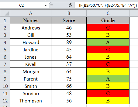
Here is a list of Names and their respective Scores.
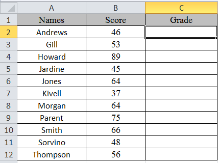
multiple if statements excel functions are used here. So, there are 3 results based on the condition. if then statements in excel is used via excel conditional formatting formula
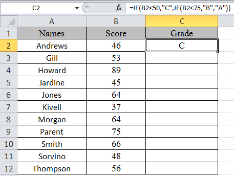
Write the formula in C2 cell.
Formula
| =IF(B2<50,"C",IF(B2<75,"B","A")) |
Explanation:
IF function only returns 2 results, one [value_if_True] and Second [value-if_False]
First IF function checks, if the score is less than 50, would get C grade, The Second IF function tests if the score is less than 75 would get B grade and the rest A grade.
Copy the formula in other cells, select the cells taking the first cell where the formula is already applied, use shortcut key Ctrl + D
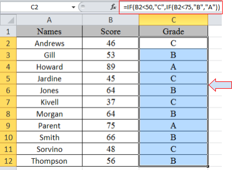
Now we will apply conditional formatting to it.
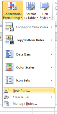
Select Home >Conditional Formatting > New Rule.
A dialog box appears
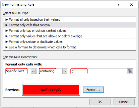
Select Format only cells that contain > Specific text in option list and write C as text to be formatted.
Fill Format with Red colour and click OK.
Now select the colour Yellow and Green for A and B respectively as done above for C.
In this article, we used IF function and Conditional formatting tool to get highlighted grade.
As you can see excel change cell color based on value of another cell using IF function and Conditional formatting tool
Hope you learned how to use conditional formatting in Excel using IF function. Explore more conditional formulas in excel here. You can perform Conditional Formatting in Excel 2016, 2013 and 2010. If you have any unresolved query regarding this article, please do mention below. We will help you.
Related Articles:
How to use the Conditional formatting based on another cell value in Excel
How to use the Conditional Formatting using VBA in Microsoft Excel
How to use the Highlight cells that contain specific text in Excel
How to Sum Multiple Columns with Condition in Excel
Popular Articles:
50 Excel Shortcut to Increase Your Productivity
How to use the VLOOKUP Function in Excel
How to use the COUNTIF function in Excel 2016
How to use the SUMIF Function in Excel
The applications/code on this site are distributed as is and without warranties or liability. In no event shall the owner of the copyrights, or the authors of the applications/code be liable for any loss of profit, any problems or any damage resulting from the use or evaluation of the applications/code.


Hi Sir/Madam,
I would like to seek your advise to create an Excel formula:
IF (a=b) & (c=d), then =e, IF NOT = 0
Kindly advise if you may. Thank you.
Write IF(AND(A=B,C=D),E,0)
I hope this helps you.
Hi Sir/Madam,
I would to know how to create a formula something like:
If (a=b) & (c=d), then = e, If not 0
Kindly advise. Thank you.
I would like the conditional formatting in one cell to be replicated in another based on the condition met in the first field. Same color coding that is.
amitabh, from your weakly detailed question without concise examples or specifics, you might be wanting or needing a conditional format "formula" ("Use a formula" choice for conditional formatting), and with absolute rather than relative references , i.e. use dollar sign(s) ($) in the formula. E.g. for A1, instead of setting the conditional format as "cell value greater than 0" make it "use a formula" with condition "=$a1>0"
Then copying A1 and "paste special" of the cell's format to B1 might achieve the result that I infer that you are interested in. The way that I set up the absolute references above, you could make B2 trip its format condition the same as A2, and B3 like A3, etc.
I'm not subscribed to the thread so anyone else is welcome to chirp in but I won't see it.
BTW, for advanced users of VBA - beware how the normally sane Microsoft developers destroyed the conditional formatting properties in Excel 2016 (and probably 07, 10, and 13; yet 03, as usual, works perfectly) when you use Formula based conditional formatting and referential addressing. Some imbecile developer (and his negligently inept reviewers) thought it would be cute to propagate .Formula1 when AppliesTo is a range with more than one cell. This was high order stupidity. Now when you copy a conditionally formatted cell (with "formula" style, and anything other than fully absolute cell designations) to a range of more than one cell, the AppliesTo of the destination all show the same (e.g. $A$2:$A$5), which is fine; but, BUT, .Formula1 shows the same thing EVERY TIME. So if you copy A1 to A2:A5, and examine .Formula1, it will say, e.g., "=A2>0" on every one of them. How mentally inept is that! In the correctly operating world (version 2003) which wasn't broken yet was fixed, .Formula1 for cell A2 would show "=A2>0" and cell A3's would be "=A3>0" and a4's would be "=A4>0". What the cutesie developers did breaks code, because .Formula1 NO LONGER REPRESENTS the correct cell address. Again, this is only for cases where AppliesTo.Count>1. The solution to this destroyed functionality (way to go, you turd that implemented this, if you haven't killed yourself yet and are reading this), is to NOT use .Formula1 in VBA as is, but rather to calculate the offsets from the first cell in .AppliesTo.Address, and apply those to .Formula1 before acting on its value. Such incompetence...yet I guarantee you that the destructive "improvement" was bragged and touted as yet another example of Microsoft making the world a better place (and you better believe that every superficial tech media writer - that's 98.8% of them - fawningly proclaimed the same, fanboying its "greatness" and the "brilliance of the tireless developers who never stop until they make Excel better"). But now you know, in one of a million examples, the actual story. Microsoft: making the world a less productive place.
how do I get the below colours using the below 2 set of conditions in the same column
+/- 10% = green
>10%20% = red
and
>-10%-20% = red
how do I get the below colours using the below 2 set of conditions in the same column
+/- 10% = green
>10% 20% = red
> -10% -20% = red
Need help with conditional formatting for the following: IF the sum of a2 thru a6 is > a1, format cells a2 thru a6 that contain numbers (with the 'bad style' (or pink fill with red font). Is this even possible?
I'm trying to use the greater than OR less than function on an =IF function cell. It doesn't work.
example
Cell value - Greater than - =$j$5
J5 is where my IF function is. I think it's reading the formula and not the final out come of the IF function which is a number
hi,
I have to enter value everyday for nest cell to last week
now if that sale value is greater then last week green colour
if not red colour
please help
Hi,
I have data as follows:
B1:F13 (5 random numbers in each row)
And another set of numbers
J1:Q2 (16 numbers)
I used conditional formatting to highlight the duplicate values.
I would appreciate if anyone can assist with an if statement that would return "1" if only 3 numbers are highlighted, 4 if 4 numbers are highlited and 10 if 5 numbers are highlighted.
Thank you
I'm trying to use conditional formatting using an IF statement to change a cell to 0 with a strikethrough if the cell is less than or equal to 0. Would anyone know how to do that if possible? Thanks in advance!
Hi Brad,
You can't change any value using conditional formatting as it will only allow you to format the range/cell based on condition entered.
In case you only want to strikenthrough the cell if negative value is entered, simply select the cell and open Conditional Formatting dialog box.
Go to "Format only cell that contain" and select "Cell Value" as "Less than or equal to" and put 0 in the input box. After that, click on Format and click on "Strikenthrough" and then hit OK twice.
You can test the condition now as it should work.
For more Excel Queries, we request you to please login on Excel Forum and post your queries there to get the instant solution for the same.
Regards,
Site Admin
I ran a conditional formatting rule to find duplicates in column A (=COUNTIF($A$1:$A$3556,$A1)>1) .... which gave me my duplicates 🙂
Now i want to run a second rule to search for duplicates in column B but but only against the highlighted rows from my conditional formatted search. ---
end result: i just want to check the duplicate rows to see if the info in column B is different.
( column A - addresses, column B first name column C last name)
I don't care about last name i need to see if there is duplicate first name record against the duplicate address result. Please help
Hi Imran,
As you mentioned that you have got the duplicates value (highlighted by conditional formatting) in column A and now you want to lookup the corresponding value whether it is duplicate or not against the highlighted value?
Here is the formula which you have to apply through conditional formatting in column B (assuming your data starts from row 2).
=COUNTIFS($A:$A,$A2,$B:$B,$B2)>1The above formula will highlight the duplicate values in column B for the highlighted duplicates value in column A.
Happy Learning,
Site Admin
Hi, i was wondering if you can conditionally format under a number of conditions. For example.
If cell a1 is less than 0.05 then format cell b2 if it is greater than 0.5, if cell a1 is 0.05-0.10, then format cell b2 if it is greater than 0.25, if cell a1 is between 0.1 and 0.5 the format cell b2 if it is greater than 0.15.....does this makes sense? Can you have multiple conditions on multiple cells for formatting on one cell?? Please help.
What if Column C had numbers (they are weekly grades), and you wanted to show a trend (arrows) comparing progress of each student from the current week (column c) from the previous week (column b)
Patrick, most font sets have arrows in them. if you go into the start menu and in the search box, type "character map". In the character map, you can copy characters and paste them into the formula. So in your case, the formula would look like:
=IF(C2>B2,"?",IF(C2=B2,"","?"))
My arrows got converted to question marks, but where you see the question marks in the formula, you would copy and paste the up and down arrows from the character map.
Thanks Obaye West
good
great
Excel Forum is a good forum for learning
Thanks for your appreciation