2 Ways to Sum by Month in Excel

Manytimes, we want to calculate some values by month. Like, how much sales was done in a perticular month. Well this can be done easily using pivot tables, but if you are trying to have a dynamic report than we can use a SUMPRODUCT or SUMIFS formula to sum by month.

Let’s start with SUMPRODUCT solution.

Here is the generic formula to get sum by month in Excel

Sum_range : It is the range that you want to sum by month.

Date_range : It is the date range that you’ll look in for months.

Month_text: It is the month in text format of which you want to sum values.

Now let’s see an example:

Example: Sum Values by Month in Excel

Here we have some value associated with dates. These dates are of Jan, Feb, and Mar month of year 2019.

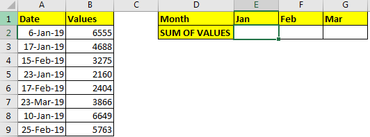
As you can see in the image above, all the dates are of year 2019. Now we just need to sum values in E2:G2 by months in E1:G1.

Now to sum values according to months write this formula in E2:

If you want to copy it in adjacent cells then use absolute references or named ranges as you in the image.

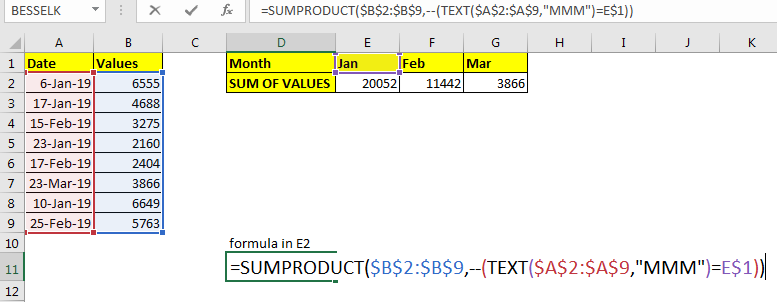
This gives us the exact sum of each month.

How it works?
Starting from the inside, let’s look at the TEXT(A2:A9,"MMM") part. Here TEXT function extracts month from each date in range A2:A9 in text format into an array. Translating to formula to =SUMPRODUCT(B2:B9,--({"Jan";"Jan";"Feb";"Jan";"Feb";"Mar";"Jan";"Feb"}=E1))

Next, TEXT(A2:A9,"MMM")=E1: Here each month in array is compared with text in E1. Since E1 contains “Jan”, each “Jan” in array is converted to TRUE and other into FALSE. This translates the formula to =SUMPRODUCT($B$2:$B$9,--{TRUE;TRUE;FALSE;TRUE;FALSE;FALSE;TRUE;FALSE})
Next --(TEXT(A2:A9,"MMM")=E1), converts TRUE FALSE into binary values 1 and 0. The formula translates to =SUMPRODUCT($B$2:$B$9,{1;1;0;1;0;0;1;0}).

Finally SUMPRODUCT($B$2:$B$9,{1;1;0;1;0;0;1;0}): the SUMPRODUCT function multiplies the corresponding values in $B$2:$B$9 to array {1;1;0;1;0;0;1;0} and adds them up. Hence we get sum by value as 20052 in E1.

SUM IF Months From Different Year

In the above example, all dates were from the same year. What if they were from different years? The above formula will sum values by month irrespective of year. For example, Jan of 2018 and Jan of 2019 will be added, if we use the above formula. Which is wrong in most of cases.

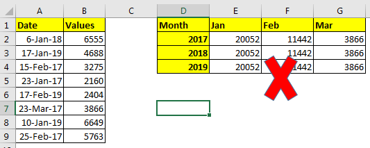
This will happen because we don’t have any criteria for the year in the above example. If we add year criteria too, it will work.

The generic formula to get sum by month and year in Excel

Here, we have added one more criterion that checks the year. Everything else is the same.
Let’s solve the above example, write this formula in cell E1 to get the sum of Jan in the year 2017.

Before copying in below cells use named ranges or absolute references. In the image, I have used named ranges for copying in the adjacent cells.

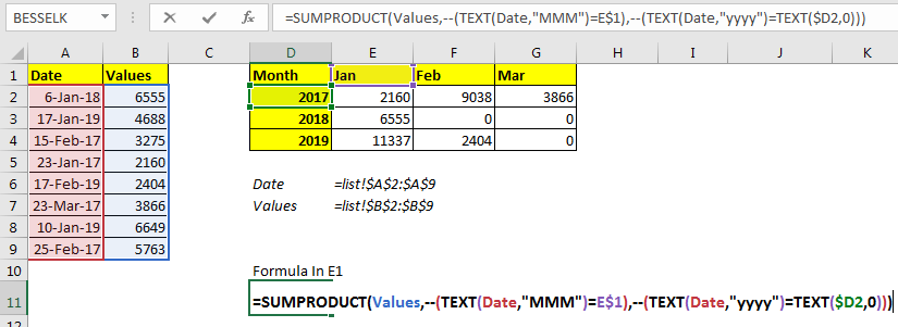
Now we can see the sum of value by months and years too.

How does it work?
The first part of formula is same as previous example. Lets understand the additional part that adds the year criteria.
--(TEXT(A2:A9,"yyyy")=TEXT(D2,0)): TEXT(A2:A9,"yyyy") converts date in A2:A9 as years in text format into an array. {"2018";"2019";"2017";"2017";"2019";"2017";"2019";"2017"}.
Most of the time, year is written in number format. To compare a number with text we, I have converted year int text using TEXT(D2,0). Next we compared this text year with array of years as TEXT(A2:A9,"yyyy")=TEXT(D2,0). This returns an array of true-false {FALSE;FALSE;TRUE;TRUE;FALSE;TRUE;FALSE;TRUE}. Next we converted true false into number using -- operator. This gives us {0;0;1;1;0;1;0;1}.
So finally the the formula will be translated to =SUMPRODUCT(B2:B9,{1;1;0;1;0;0;1;0},{0;0;1;1;0;1;0;1}). Where first array is values. Next is matched month and third is year. Finally we get our sum of values as 2160.

Using SUMIFS function to sum by Month

Generic Formula

Here, Sum_range : It is the range that you want to sum by month.

Date_range : It is the date range that you’ll look in for months.

Startdate : It is the start date from which you want to sum. For this example, it will be 1st of the given month.

Example: Sum Values by Month in Excel
Here we have some value associated with dates. These dates are of Jan, Feb, and Mar month of year 2019.

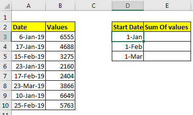
We just need to sum these values by there month. Now it was easy if we had months and years separately. But they are not. We can’t use any helping column here.
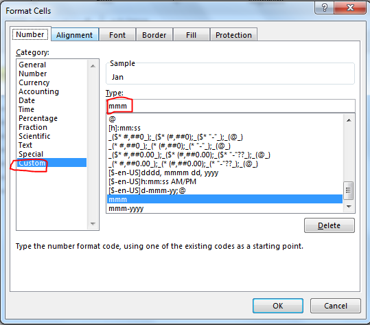
So to prepare report, I have prepared a report format that contains month and sum of values. In the month column, I actually have a start date of the month. To Just see the month, select start date and press CTRL+1.
In custom format, write “mmm”.


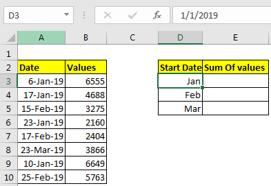
Now we have our data ready. Let’s sum the values by month.

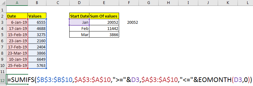
Write this formula in E3 to sum by month.

Use absolute references or named ranges before copying down the formula.

So, finally we got the the result.

So, How it Works?

As we know that SUMIFS function can sum values on multiple criterias.
In example above, the first criteria is sum all values in B3:B10 where, date in A3:A10 is greater than or equal to date in D3. D3 contains 1-Jan. This translates too.

Next Criteria is sum only if Date in A3:A10 is less than or equal to EOMONTH(D3,0). EOMONTH Function just returns serial number of last date of month provided. Finally formula translates too.

Hence, we get the sum by month in excel.

Benefit of this method is that you can adjust the start date for summing the values.

If your dates have different years than it is best to use pivot tables. Pivot tables can help you segregate the data in yearly, quarterly and monthly format is easily.

So yeah guys, this is how you can sum values by month. Both ways have their own specialities. Choose which way you like.

If you have any queries regarding this article or any other excel and VBA related queries, the comments section is open for you.

Relate Articles:
How to Use SUMIF Function in Excel
SUMIFS with dates in Excel
SUMIF with non-blank cells
How to Use SUMIFS Function in Excel
SUMIFS using AND-OR logic

Popular Articles

50 Excel Shortcut to Increase Your Productivity: Get faster at your task. These 50 shortcuts will make you work even faster on Excel.

How to use the VLOOKUP Function in Excel: This is one of the most used and popular functions of excel that is used to lookup value from different ranges and sheets.

How to use the COUNTIF function in Excel: Count values with conditions using this amazing function. You don't need to filter your data to count specific values. Countif function is essential to prepare your dashboard.

How to use the SUMIF Function in Excel: This is another dashboard essential function. This helps you sum up values on specific conditions.