
In this article, we will learn how to get the Average with multiple criteria in Excel.
Problem?
For Instance, We have a large list of data and we need to find the Average of the price or amount given some criteria. Criteria can be applied over any column of the data.
How to solve the Problem.
Now we will make a formula out of the function. Here we are given the data and we needed to find the AVERAGE of the numbers having some criteria
Generic formula:
Notes: do not provide date directly to the function. Use DATE function or use cell reference for date argument in excel as Excel reads date only with the correct order.
Example:
All of these might be confusing to understand. So, let's test this formula via running it on the example shown below.
Here we have given data from A1:D51. We need to find the AVERAGE of Quantity received as per different criteria.
Conditions are as follows.
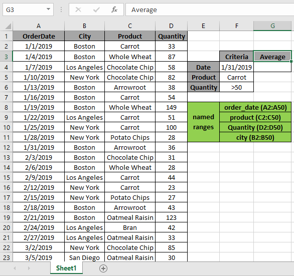
The above 4 stated conditions or criteria needs to be matched. The AVERAGEIFS function can help us extract the average having different criteria.
Use the Formula:
Quantity : named range used for D2:D50 array
Order_date : named range used for A2:A50 array
City : named range used for B2:B50 array
Product: named range used for C2:C50 array
F4 : cell reference used for criteria 1
F5 : cell reference used for criteria 2
F6 : cell reference used for criteria 3
Explanation:
Here the A2 is given as cell reference & Named ranges given as rng ( D2 : D51 ) and order_date ( A2 : A51).
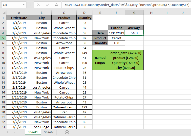
As you can see in the above snapshot the AVERAGE of the quantity in January comes out to be 54.00. As there is only one value satisfying all conditions.
Example 2:
Here we have given data from A1:D51. We need to find the AVERAGE of Quantity received as per different criteria.
Conditions are as follows.
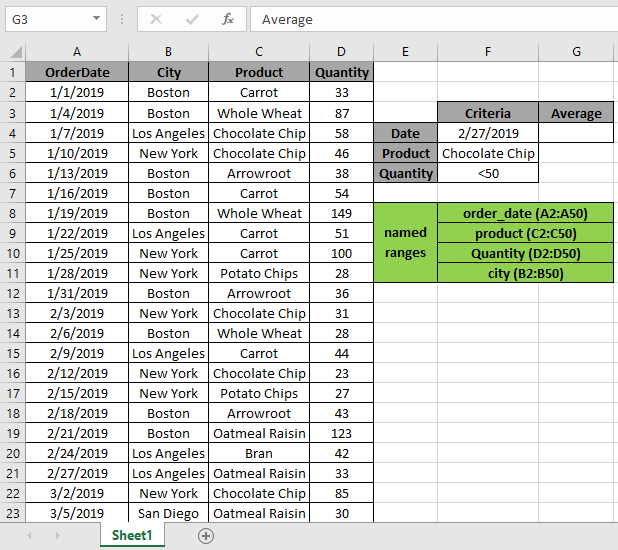
The above 4 stated conditions or criteria needs to be matched. The AVERAGEIFS function can help us extract the average having different criteria.
Use the Formula:
Quantity : named range used for D2:D50 array
Order_date : named range used for A2:A50 array
City : named range used for B2:B50 array
Product: named range used for C2:C50 array
F4 : cell reference used for criteria 1
F5 : cell reference used for criteria 2
F6 : cell reference used for criteria 3
Explanation:
Here the A2 is given as cell reference & Named ranges given as rng ( D2 : D51 ) and order_date ( A2 : A51).
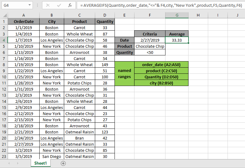
As you can see in the above snapshot the AVERAGE of the quantity in January comes out to be 33.33... As there is only one value satisfying all conditions.
Here are some observations about the formula usage below.
Notes:
Hope this article about how to Average with multiple criteria in Excel is explanatory. Find more articles on SUMPRODUCT functions here. Please share your query below in the comment box. We will assist you.
Related Articles
How to use the AVERAGEIFS function in excel
How to use the DAVERAGE Function in Excel
How To Highlight Cells Above and Below Average Value
Ignore zero in the Average of numbers
Average Difference between lists
Create drop down list in excel with colour
Popular Articles
If with conditional formatting
Join first and last name in excel
Count cells which match either A or B
The applications/code on this site are distributed as is and without warranties or liability. In no event shall the owner of the copyrights, or the authors of the applications/code be liable for any loss of profit, any problems or any damage resulting from the use or evaluation of the applications/code.


