Data extraction and cleaning is the first and most crucial task of any data analysis project. In my five years of experience, I have received data that looked like garbage, but using excel RIGHT and LEFT functions I was able to turn them into meaningful reports.
Data cleaning in excel is easy. Here I am going to explain how you can extract specific text in excel 2016 from a cell and leave behind garbage data.

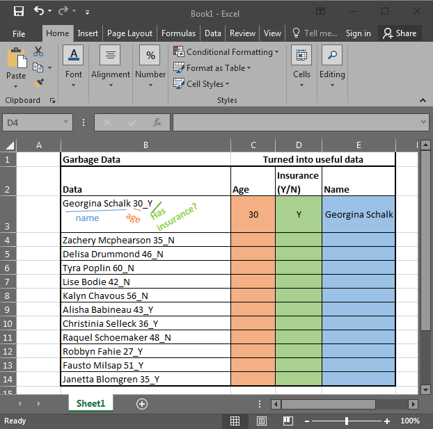
In the above image, I am provided with data in Excel. It has Name, Age, and if the person has any insurance or no (Y/N). To use this data, I need to extract data in different columns. Each column should contain only one kind of value. Once it’s done we can make pivot reports in excel that will tell us better about the data. So let's get started.
Let’s start with the easiest one. In this example, we have “Has insurance?” data at the end of the string. And that is only one character (Y or N). To extract this data we will use the RIGHT Formula Excel provides. The RIGHT function is available in Excel 2016, Excel 2013, Excel 2010 and older versions of Excel.

RIGHT function in excel takes only two arguments. First the TEXT, and second the NUMBER OF CHARACTERS you want to extract from the right in excel.
Generic Formula:
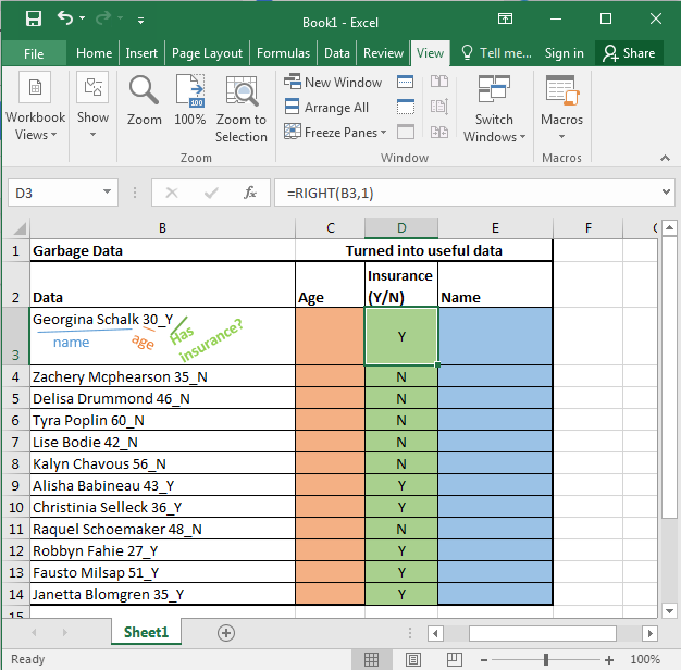
Here, we have our text in cell B3 and the number of characters we want to extract is 1. Just write this formula in excel in cell D3 or wherever you want to have this data.
You will have your result in cell D3. just copy or drag down this formula in the cells below.
Now let's get our age. Before explaining, let me show you the formula. Copy this formula in desired cells.
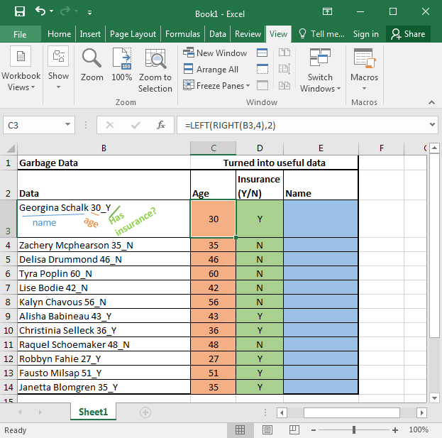
In the above formula, we have combined LEFT and RIGHT functions to get our specific text from the string. This is how it looks.

Now let's understand this puny formula.
Every function works from inwards to outwards. So let's start with:
RIGHT(B3,4): It simply extracts 4 characters from a given text. That gives us 30_Y. Why 4? Since we know that age is only one of two characters, and we have 1 “_” and 1 Y or N.
LEFT(RIGHT(B3,4),2): Now we have our text that starts with age that is of 2 characters. Here comes the LEFT function into action. It takes RIGHT(B3,4) as its text argument and extracts 2 characters from that. That gives us 30 for the first cell. Copy the formula in the cells below and you will get the rest of the data as shown in the image above.
Generic Formula for LEFT:
Just like the RIGHT function in excel LEFT function of Excel also takes two same arguments. It just extracts data from the left of the string provided.
Just paste this formula in desired cells to extract the name from the text in excel.
In the above examples, we knew the exact number of texts to extract from the given text. But now, we don’t know how lengthy a name is. What can be done?
We do know that the name is followed by exact 5 characters. 1 for space, 2 for the age, 1 for “_” underscore, and one for the Y.
If we can get all number of text and then subtract 5 from that then we will have the exact number of text for the name.
For finding the length of a text in Excel we can use the LEN function. The LEN function of excel returns the number of characters involved.
Syntax:
So LEN(B3) returns 20.
LEN(B3)-5 returns 15. And this the length of the name in cell B3
At last LEFT(B3, LEN(B3)-5) gives us Georgina Schalk as a result. When you copy the formula in the cells below, you get all the names.
Now you can prepare reports like this based on extracted data using pivot tables. It tells us that half of our subjects have insurance and the other half don’t.

LEFT and RIGHT FUNCTION of excel is very powerful and useful for data cleaning. When combined with LEN function, FIND function and SUBSTITUTE function of excel they can extract any substring within a string in excel.
In future, we will see more complex data extraction in excel. For now bye. And yes, leave your thoughts in the comments section below. I will be more than happy to help you.
The applications/code on this site are distributed as is and without warranties or liability. In no event shall the owner of the copyrights, or the authors of the applications/code be liable for any loss of profit, any problems or any damage resulting from the use or evaluation of the applications/code.
I have a SA ID number consisting of 13 digits. I only want excel to extract the first 6 numbers of the ID number but I also need hyphens between the first 2 numbers and between the next 2 numbers. My formula is =LEFT(F6 6) where F6 is the cell address. Please help. thanks.