
In this article, we will learn How to use the AVERAGEIF function in Excel.
AVERAGE or MEAN based on criteria
In EXCEL, while working with mean values or generally called as average of values. Then we use AVERAGE function. But if we have a criteria to match, so use AVERAGEIF function. Use the AVERAGEIFS function to match multiple criteria. Let's understand how AVERAGEIF function syntax and some example to illustrate the function usage.
AVERAGEIF Function in Excel
AVERAGEIF function commutes the average of the array that meets the supplied SINGLE statement.
AVERAGEIF Function Syntax:
| =AVERAGEIF (range, criteria, [average_range]) |
range : where criteria is applied.
criteria : condition to be applied
[average range] : [optional] range where the average need to be calculated, if it is different from the first range provided as argument
Example :
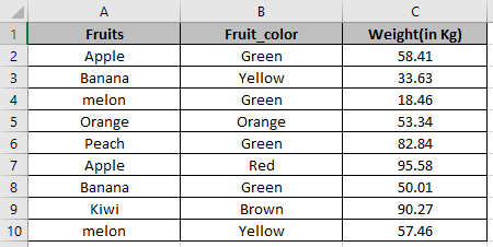
All of these might be confusing to understand. Let's understand how to use the function using an example. Here we have a list of fruits with color and their weight.
First we will find out the average of overall weight of the fruits having condition <50 Kg.
Use the formula
| =AVERAGEIF(C2:C10,"<50") |
C2:C10 : range where condition (cell_value<50) satisfies.
<50: condition or criteria
C2:C50 : the average range as no other range is provided.
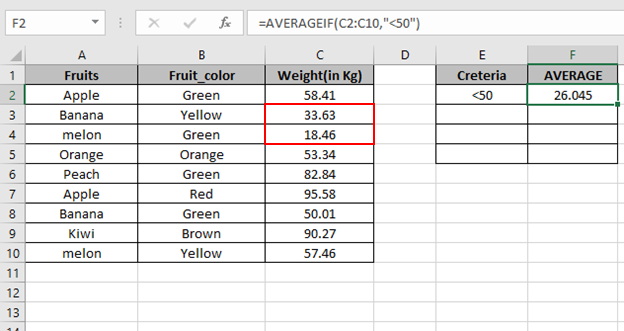
We got the Average of the cells less than 50.
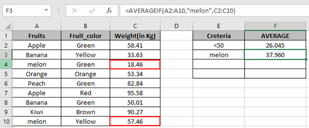
Now we will compute the Average of the weight having fruit melon.
Use the formula
| =AVERAGEIF(A2:A10,"melon",C2:C10) |

We got the Average of the cells in colored box.
Now we will compute the Average of the weight not having fruit Banana
Use the formula
| =AVERAGEIF(A2:A10,"<>Banana",C2:C10) |
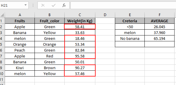
We got the Average of the cells in Red colored box.
Now we will compute the Average of the weight having multiple conditions. We need to use AVERAGEIFS function.
Conditions
Use the formula
| =AVERAGEIFS(C2:C10, A2:A10,"Apple", B2:B10,"Red") |
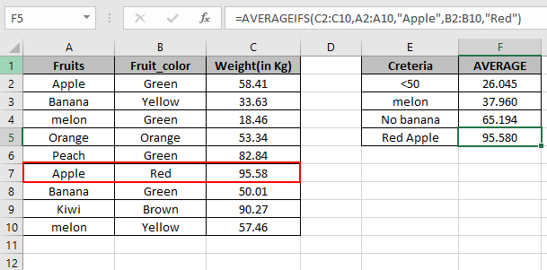
As you can see your Average is here.
Ignore Zero in list using AVERAGEIF function
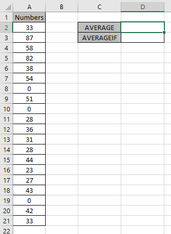
Here we are given a list of numbers and we need to find the average of numbers where zeroes are ignored and rest are considered.

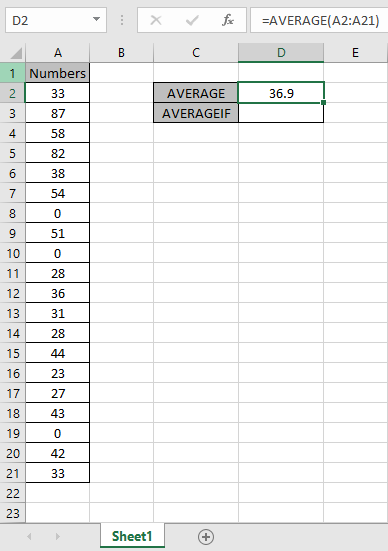
First of all we need Average of the numbers including zeroes.

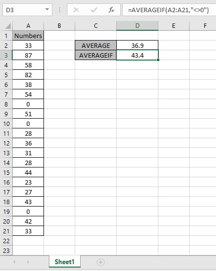
This formula will accept values except zero.
Use the formula:
| =AVERAGEIF(A2:A21, "<>0") |
A2:A21 : range
“<>0” : condition for ignoring zero values.

As you can see the difference in the values. The Average of the numbers ignoring zero is 43.4.
For Blank cells
One more thing that is to understand is the AVERAGE, AVERAGEIF & AVERAGEIFS function ignores blank cells (and cells that contain text values). So there is no need to filter results.
AVERAGEIF with months criteria
Here we have a data from A1:D51. we need to find the AVERAGE of Quantity in the month of January.
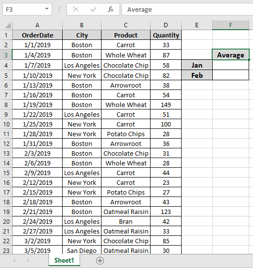
First we will find a date which has the first date of the month which is the A2 cell. Named ranges are rng ( D2 : D51 ) and order_date ( A2 : A51).
Use the Formula:
| = AVERAGEIFS ( rng , order_date , ">=" & A2 , order_date , "<=" & EOMONTH ( A2 , 0 ) ) |
Explanation:
{ 33 ; 87 ; 58 ; 82 ; 38 ; 54 ; 149 ; 51 ; 100 ; 28 ; 36 }
Here the A2 is given as cell reference & Named ranges given as rng ( D2 : D51 ) and order_date ( A2 : A51).
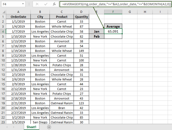
As you can see in the above snapshot the AVERAGE of the quantity in January comes out to be 65.091 .
Now we will get the AVERAGE of the quantity in February by changing the First date argument of the function
Use the Formula:
| = AVERAGEIFS ( rng , order_date , ">=" & A13 , order_date , "<=" & EOMONTH ( A13 , 0 ) ) |
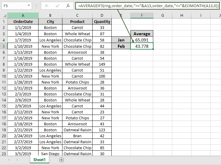
As you can see in the above snapshot the AVERAGE of the quantity in January comes out to be 43.778 .
AVERAGE and AVERAGEIF Example :
Here Let’s understand this function using it in an example.
First of all we need Average of the numbers including zeroes.
This formula will accept values except zero.
Use the formula:
| =AVERAGEIF(A2:A21, "<>0") |
A2:A21 : range
“<>0” : condition for ignoring zero values.
As you can see the difference in the values. The Average of the numbers ignoring zero is 43.4.
If you don't have any zero value in the array. You can use the return zero out of all the error values and use the formula how to take the average of numbers ignoring zeros here. But this formula doesn't work with error values.
Here are all the observational notes using the AVERAGEIF function in Excel
Notes :
Hope this article about How to use the AVERAGEIF function in Excel is explanatory. Find more articles on calculating values and related Excel formulas here. If you liked our blogs, share it with your friends on Facebook. And also you can follow us on Twitter and Facebook. We would love to hear from you, do let us know how we can improve, complement or innovate our work and make it better for you. Write to us at info@exceltip.com.
Related Articles :
How To Highlight Cells Above and Below Average Value : highlight values which are above or below the average value using the conditional formatting in Excel.
Ignore zero in the Average of numbers : calculate the average of numbers in the array ignoring zeros using AVERAGEIF function in Excel.
Calculate Weighted Average : find the average of values having different weight using SUMPRODUCT function in Excel.
Average Difference between lists : calculate the difference in average of two different lists. Learn more about how to calculate average using basic mathematical average formula.
Average numbers if not blank in Excel : extract average of values if cell is not blank in excel.
AVERAGE of top 3 scores in a list in excel : Find the average of numbers with criteria as highest 3 numbers from the list in Excel
Popular Articles :
How to use the IF Function in Excel : The IF statement in Excel checks the condition and returns a specific value if the condition is TRUE or returns another specific value if FALSE.
How to use the VLOOKUP Function in Excel : This is one of the most used and popular functions of excel that is used to lookup value from different ranges and sheets.
How to Use SUMIF Function in Excel : This is another dashboard essential function. This helps you sum up values on specific conditions.
How to use the COUNTIF Function in Excel : Count values with conditions using this amazing function. You don't need to filter your data to count specific values. Countif function is essential to prepare your dashboard.
The applications/code on this site are distributed as is and without warranties or liability. In no event shall the owner of the copyrights, or the authors of the applications/code be liable for any loss of profit, any problems or any damage resulting from the use or evaluation of the applications/code.


