Shortcut to open drop down filter in Excel

In this article, we will learn the shortcut to open a filter drop-down list and the filter in Ribbon in Microsoft Excel.

“Auto Filter” option allows us to filter the data based on content of cells and conditions applied on them.

We can filter the according to the particular text, month, date, number, cell color, font color, etc. Even we can sort the data as per the number, text, cell colors, and font colors, etc.

This option is available in the Data Tab under the Sort & Filter group.
 

 
Excel filter shortcut Key:- Press Ctrl+Shift+L on your keyboard.
 
Let’s take an example to understand how we can filter the data using shortcut keys.

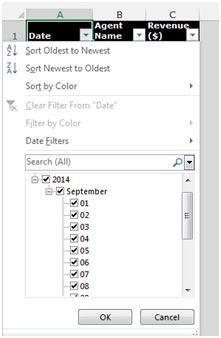
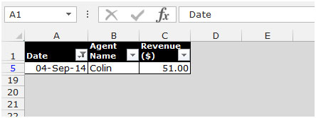
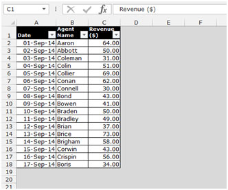
We have data in range A1: C18. Column A contains Date, column B contains Agent name, and column C contains Revenue amount.
 

 
Filter the data through Short cut key

Follow below given steps:-

• Select the first cell of data.
• Press the key Ctrl+Shift+L on your keyboard.

• If you want to put the data as per date.
• Click on the filter with the mouse.
• Drop down list will appear.

• Select any date from the list.

• Only selected date’s related data will be appear.
• We can follow the same procedure for Agent Name list and Revenue list.

 
Filter the data through Short cut key

Follow below given steps:-

• Select the first cell of data.
• Go to the Data Tab, click on Filter from the Sort & Filter group.

• If you want to put the data as per date.
• Click on the filter with the mouse.
• Drop down list will appear.
• Select any date from the list.

• Only selected date’s related data will appear.

• We can follow the same procedure for Agent Name list and Revenue list.

These are the ways we can put the filter by using the shortcut key and from ribbon in Microsoft excel.

If you liked our blogs, share it with your friends on Facebook. And also you can follow us on Twitter and Facebook.
We would love to hear from you, do let us know how we can improve, complement or innovate our work and make it better for you. Write us at info@exceltip.com