
In this article, we will learn How to Sum using Text Characters as Criteria in Excel.
Sum with some criteria
Whenever we need to find the sum of values having criteria, we use the SUMIF function. It lets the user have the sum of values having criteria on the corresponding text values. For example finding the sum of price of products which belong to the household category. We know how to sum one column on multiple conditions. We use the SUMIFS function. But how do we sum multiple columns in one condition. This article is all about summing multiple columns on condition.
SUMIF Formula with wildcard in Excel
Generic Formula
| =SUMPRODUCT((criteria_range=criteria)*(sum_range)) |
Criteria_range: This is the range in which criteria will be matched.
Criteria: this is the criteria or condition.
Sum_range: the sum range. This can have multiple columns but same rows as criteria range.
Example :
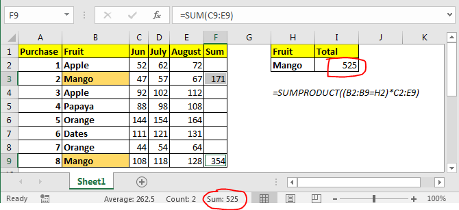
In the above image, we have this table of the amount spent on different fruits in different months. We just need to get the total amount spent on mangoes in all these months.
In I2 the formula is
| =SUMPRODUCT((B2:B9=H2)*C2:E9) |
This returns 525 as total amount spent on mangos. You can see this in image above.
How does it work?
Well, it is easy. Let’s break down the formula and understand it in pieces.
(B2:B9=H2): This part compares each value in range B2:B9 with H2 and returns an array of TRUE and FALSE. {FALSE;TRUE;FALSE;FALSE;FALSE;FALSE;FALSE;TRUE}.
(B2:B9=H2)*C2:E9: Here we multiplied each value in the above array with values in C2:E9. C2:C9 are also treated as an 2D array. Finally this statement returns a 2D array of {0,0,0;47,57,67;0,0,0;0,0,0;0,0,0;0,0,0;0,0,0;108,118,128}.
Now SUMPRODUCT looks like this SUMPRODUCT({0,0,0;47,57,67;0,0,0;0,0,0;0,0,0;0,0,0;0,0,0;108,118,128}). It has values of mango only. It sums them up and returns the result as 525.
Another method can be having a totals column and then use it with SUMIF function to get the sum of all columns. But that’s not what we want to do.
SUMIF Function in Excel
As the name suggests, the SUMIF formula in Excel sums values in a range on a given condition.

Generic Excel SUMIF Formula:
| =SUMIF(condition_range,condition,sum range) |
Let's jump into an example. But theory…, Ah! We will cover it later.
Use SUMIF To Sum Values On One Condition
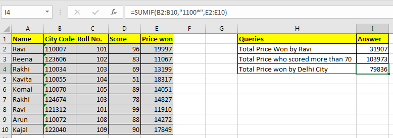
For this example I have prepared this data.
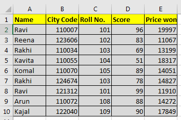
Based on this data we need to answer these questions:
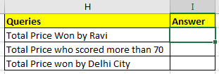
Let's start with the first question.
SUMIF with Text Condition
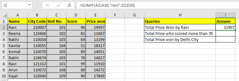
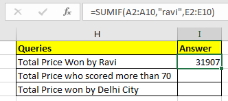
We need to tell the sum of the price won by Ravi.
So our condition range will be name range and that is A2:A10.
Our condition is Ravi and
Sum range is E2:E10.
So in cell I2 we will write:
| =SUMIF(A2:A10,"ravi",E2:E10) |
Note that ravi is in double quotes. Text conditions are always written in double quotes. This is not the case with numbers.
Note that ravi is written in all smalls. Since SUMIF is not case sensitive, hence it doesn’t matter.
The above SUMIF formula will return 31907 as shown in the image below.
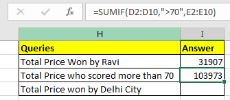
SUMIF with Logical Operators
For the second question, our condition range will be D2:D10.
Condition is >70 and
The sum range is the same as before.
| =SUMIF(D2:D10,">70",E2:E10) |
The above SUMIF formula will return 103973 as shown in the image below.
SUMIF with Wild Card Operators
In the third question, our condition is Delhi. But we don’t have a city column. Hmmm… So what do we have? Aha! City code. This will work.
We know that all Delhi city codes start from 1100. City codes are in 6 digits. So we know it is 1100??. “?” operator is used when we know number of characters but don’t know the character. As here we know that there are two more numbers after 1100. They can be anything, so we used “?”. If didn’t know the number of characters, we would use “*”.
Remember wild card operators only work with text values. Hence you need to convert city code into text.
You can concatenate numbers with “” to make them text value.
| (formula to convert number into text) = number & “” or =CONCATENATE(number,””) |
Now in cell I2 write this formula
| =SUMIF(B2:B10,"1100??",E2:E10) |
This will return the sum of the price whose city code starts with 1100. In our example it is 79836.
Observational Notes:
Hope this article about How to Sum using Text Characters as Criteria in Excel is explanatory. Find more articles on calculating values and related Excel formulas here. If you liked our blogs, share it with your friends on Facebook. And also you can follow us on Twitter and Facebook. We would love to hear from you, do let us know how we can improve, complement or innovate our work and make it better for you. Write to us at info@exceltip.com.
Related Articles :
Replace text from end of a string starting from variable position: To replace text from the end of the string, we use the REPLACE function. The REPLACE function uses the position of text in the string to replace.
How to Check if a cell contains one of many texts in Excel: To find check if a string contains any of multiple text, we use this formula. We use the SUM function to sum up all the matches and then perform a logic to check if the string contains any of the multiple strings.
Count Cells that contain specific text: A simple COUNTIF function will do the magic. To count the number of multiple cells that contain a given string we use the wildcard operator with the COUNTIF function.
Popular Articles :
How to use the IF Function in Excel : The IF statement in Excel checks the condition and returns a specific value if the condition is TRUE or returns another specific value if FALSE.
How to use the VLOOKUP Function in Excel : This is one of the most used and popular functions of excel that is used to lookup value from different ranges and sheets.
How to use the SUMIF Function in Excel : This is another dashboard essential function. This helps you sum up values on specific conditions.
How to use the COUNTIF Function in Excel : Count values with conditions using this amazing function. You don't need to filter your data to count specific values. Countif function is essential to prepare your dashboard.
The applications/code on this site are distributed as is and without warranties or liability. In no event shall the owner of the copyrights, or the authors of the applications/code be liable for any loss of profit, any problems or any damage resulting from the use or evaluation of the applications/code.


I found this tip to be just what I needed when trying to pick out cells that contained dates and then summing the associated values. My problem was that I wanted only the various dates and not the cells that contained other text. I found that by using "*/*" the =SUMIF would extract only the cells containing the dates. Absolutely perfect and I am so grateful!!! Shirlene