
Finding last used row and column is one of the basic and important task for any automation in excel using VBA. For compiling sheets, workbooks and arranging data automatically, you are required to find the limit of the data on sheets.
This article will explain every method of finding last row and column in excel in easiest ways.
1. Find Last Non-Blank Row in a Column using Range.End
Let’s see the code first. I’ll explain it letter.
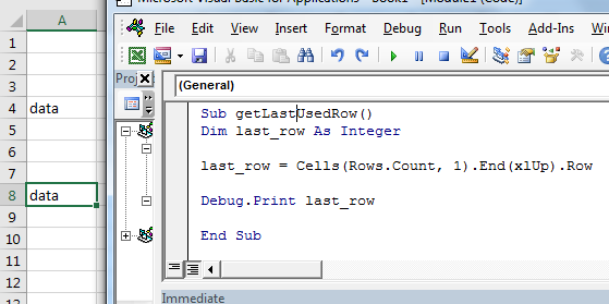
Sub getLastUsedRow()

    Dim last_row As Integer

    last_row = Cells(Rows.Count, 1).End(xlUp).Row ‘This line gets the last row

    Debug.Print last_row

End Sub
The the above sub finds the last row in column 1.
How it works?
It is just like going to last row in sheet and then pressing CTRL+UP shortcut.
Cells(Rows.Count, 1): This part selects cell in column A. Rows.Count gives 1048576, which is usually the last row in excel sheet.
Cells(1048576, 1)
.End(xlUp): End is an method of range class which is used to navigate in sheets to ends. xlUp is the variable that tells the direction. Together this command selects the last row with data.
Cells(Rows.Count, 1).End(xlUp)
.Row : row returns the row number of selected cell. Hence we get the row number of last cell with data in column A. in out example it is 8.
See how easy it is to find last rows with data. This method will select last row in data irrespective of blank cells before it. You can see that in image that only cell A8 has data. All preceding cells are blank except A4.
Select the last cell with data in a column
If you want to select the last cell in A column then just remove “.row” from end and write .select.
Sub getLastUsedRow()

Cells(Rows.Count, 1).End(xlUp).Select ‘This line selects the last cell in a column

End Sub
The “.Select” command selects the active cell.
Get last cell’s address column
If you want to get last cell’s address in A column then just remove “.row” from end and write .address.
Sub getLastUsedRow()

add=Cells(Rows.Count, 1).End(xlUp).address ‘This line selects the last cell in a column
Debug.print add
End Sub
The Range.Address function returns the activecell’s address.
Find Last Non-Blank Column in a Row
It is almost same as finding last non blank cell in a column. Here we are getting column number of last cell with data in row 4.
Sub getLastUsedCol()

    Dim last_col As Integer

    last_col = Cells(4,Columns.Count).End(xlToLeft).Column ‘This line gets the last column

    Debug.Print last_col

End Sub
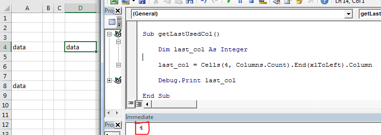
You can see in image that it is returning last non blank cell’s column number in row 4. Which is 4.
How it works?
Well, the mechanics is same as finding last cell with data in a column. We just have used keywords related to columns.
Select Data Set in Excel Using VBA
Now we know, how to get last row and last column of excel using VBA. Using that we can select a table or dataset easily. After selecting data set or table, we can do several operations on them, like copy-paste, formating, deleting etc.
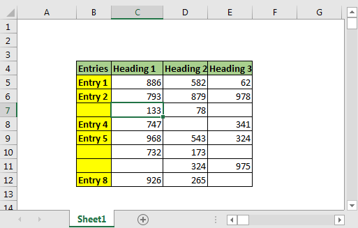
Here we have data set. This data can expand downwards. Only the starting cell is fixed, which is B4. The last row and column is not fixed. We need to select the whole table dynamically using vba.
VBA code to select table with blank cells
Sub select_table()
Dim last_row, last_col As Long

'Get last row
last_row = Cells(Rows.Count, 2).End(xlUp).Row

'Get last column
last_col = Cells(4, Columns.Count).End(xlToLeft).Column

'Select entire table
Range(Cells(4, 2), Cells(last_row, last_col)).Select

End Sub
When you run this, entire table will be selected in fraction of a second. You can add new rows and columns. It will always select the entire data.
Benefits of this method:
Cons of Range.End method:
2. Find Last Row Using Find() Function
Let’s see the code first.
Sub last_row()

   lastRow = ActiveSheet.Cells.Find("*", searchorder:=xlByRows, searchdirection:=xlPrevious).Row

   Debug.Print lastRow

End Sub

As you can see that in image, that this code returns the last row accurately.
How it works?
Here we use find function to find any cell that contains any thing using wild card operator "*". Asterisk is used to find anything, text or number.
We set search order by rows (searchorder:=xlByRows). We also tell excel vba the direction of search as xlPrevious (searchdirection:=xlPrevious). It makes find function to search from end of the sheet, row wise.

Once it find a cell that contains anything, it stops. We use the Range.Row method to fetch last row from active cell.
Benefits of Find function for getting last cell with data:
Cons of Find() function:
3. Using SpecialCells Function To Get Last Row
The SpecialCells function with xlCellTypeLastCell argument returns the last used cell. Lets see the code first
Sub spl_last_row_()
lastRow = ActiveSheet.Cells.SpecialCells(xlCellTypeLastCell).Row
Debug.Print lastRow
End Sub
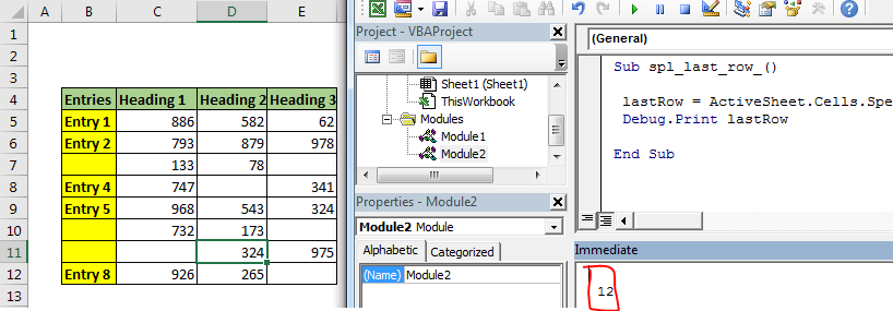
If you run the above code, you will get row number of last used cell.
How it Works?
This is the vba equivalent of shortcut CTRL+End in excel. It selects the last used cell. If record the macro while pressing CTRL+End, you will get this code.
Sub Macro1()
'
' Macro1 Macro
'

'
    ActiveCell.SpecialCells(xlLastCell).Select
End Sub
We just used it to get last used cell’s row number.
Note: As I said above, this method will return the last used cell not last cell with data. If you delete the data in last cell, above vba code will still return the same cells reference, since it was the “last used cell”. You need to save the document first to get last cell with data using this method.
Related Articles:
Delete sheets without confirmation prompts using VBA in Microsoft Excel
Add And Save New Workbook Using VBA In Microsoft Excel 2016
Display A Message On The Excel VBA Status Bar
Turn Off Warning Messages Using VBA In Microsoft Excel 2016
Popular Articles:
The applications/code on this site are distributed as is and without warranties or liability. In no event shall the owner of the copyrights, or the authors of the applications/code be liable for any loss of profit, any problems or any damage resulting from the use or evaluation of the applications/code.


