
Microsoft Excel having so many unbelievable capabilities that are not instantlyperceived. It is such a powerful spreadsheet and data analysis application, in which shortcut keys are most useful and powerful way to save the time.
Shortcut keys help to provide an easier and usually quicker method of directing and finishing commands in Microsoft Excel. Mostly we prefer to use the shortcuts as it’s kind of amazing how much time we can save by not using the mouse clicks. Shortcut keys are commonly accessed by using the Option, Control, Shift, Function key and Command key.
In this article we are providing you the Keyboard shortcuts Mac. By using you can save your time and increase the productivity as well.
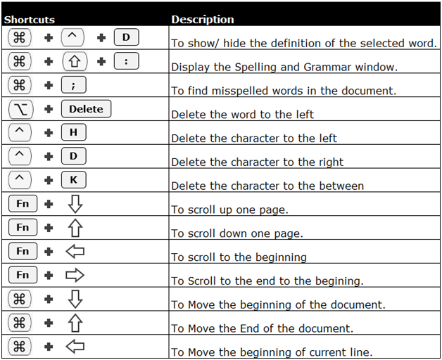
Document’s Keyboard Shortcuts:-
Finder Keyboard Shortcuts:-
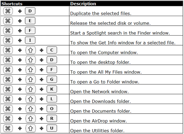
General Shortcut keys:-


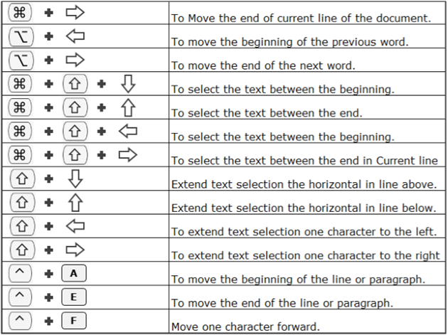
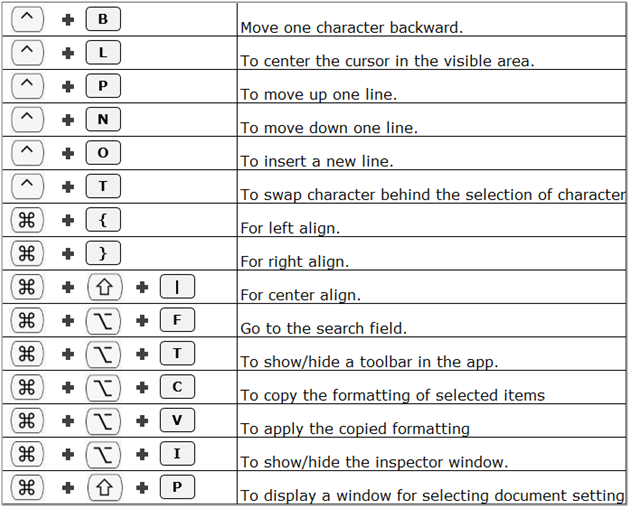
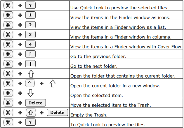
Navigating Shortcut Keys:-
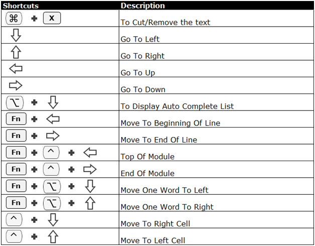

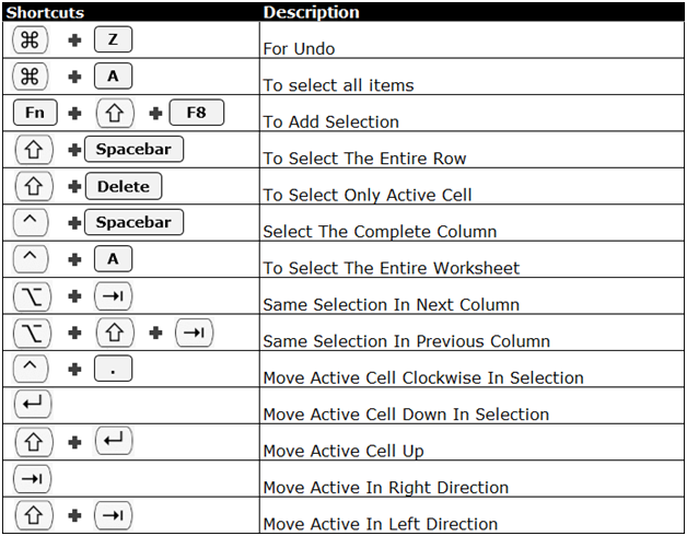
Keyboard shortcuts for selecting rows/column/cell:-
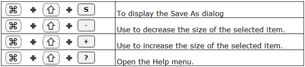
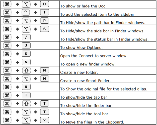
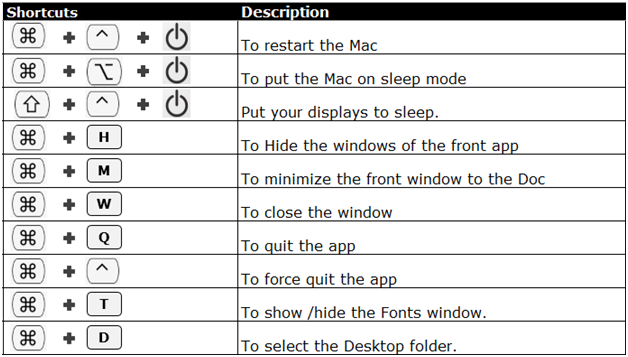
Window Keyboard Shortcuts:-
The applications/code on this site are distributed as is and without warranties or liability. In no event shall the owner of the copyrights, or the authors of the applications/code be liable for any loss of profit, any problems or any damage resulting from the use or evaluation of the applications/code.


thank you
Thank you!
Thank you!
It would be helpful to have the keyboard symbols defined.
Thank you!
Thank you for this. It's a pity there isn't a keyboard shortcut for subscript and superscript ... unless I've missed it!
Good stuff but it seems your left/up and right/down icons are swapped in at least three places. Hope this does not reflect on the accuracy of the table.
Also you have missed some of the 'most useful (IMVHO). Namely the Command Option Shift 4 and COS3 for copy selected or full screen image to clipboard.
BobJordanB
thank you, thank you, thank you, Thank You! 😀
really helpful, Thanks a lot.
Thanks for listening to us Mac fans. Much appreciated.
Excellent.
Excellent, thank you
Fantastic!!
Just need an updated excel for Mac's now!
That is very useful
This will be very handy.
Good info
Really helpful information...
there you go. now this is what we all wanted (mac version).