
In this article, we will learn how to apply nesting formulas. Through Nested formula, we can check the multiple conditions in a cell for 64 conditions. It is very useful to get the answer in a cell on the basis of different criteria. Let’s take an example to understand how we can use Nesting formulas.
We have 2 Excel data. In the 2nd data, we want to match all the columns from the second data accordingly. Also, we want to mention the comparison remarks in the 2nd data as it is showing in the below images. 1st Sheet:- 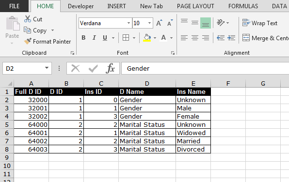 2nd Sheet:-
To resolve this query, we use a combination of formulas: - “IF”, “ISNA”, “MATCH” and “ISNUMBER”.
“IF” function used to check the logical test and also it provides the condition if value is true then what will be there. If the value will not be the same in sheet 1 then function will give the error.
“ISNA” function is used to provide the value for error.
“ISNUMBER” function: If the match values will be matched from the sheet 1 values then with the help of “IF” condition, we can provide the status for the true and false.
“MATCH” function is a key function to this formula. Through this function, we will check whether the data is same or not in the rows.
Let’s see how we will use this function in data. Follow below given steps:-
=IF(ISNA(MATCH(B2,Sheet1!$B$2:$B$8,0)),"New",IF(ISNUMBER(MATCH(A2&B2&C2&D2&E2, Sheet1!$A$2:$A$8&Sheet1!$B$2:$B$8&Sheet1!$C$2:$C$8&Sheet1!$D$2:$D$8&Sheet1!$E$2:$E$8,0)),"No change required”, “Investigation required"))
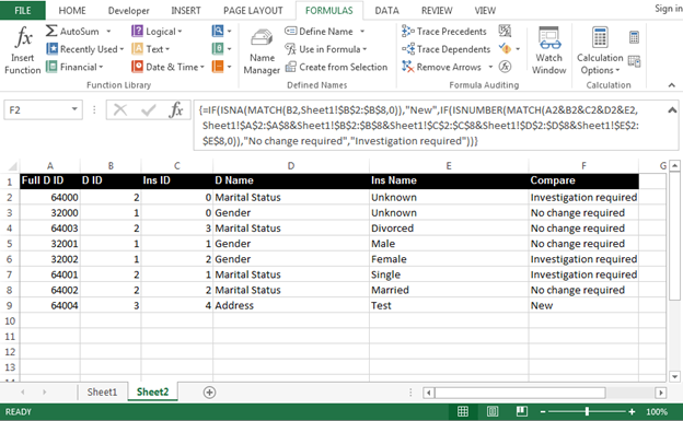
Note:- This is an Array Formula which is confirmed by pressing CTRL+SHIFT+ENTER to activate the array. You will know the array is active when you see curly brackets { } appear around your formula. If you do not press CTRL+SHIFT+ENTER, you will get an error or a clearly incorrect answer. Press F2 on that cell and try again.
This is the way we can use NESTING formulas in Microsoft Excel.
![]()
The applications/code on this site are distributed as is and without warranties or liability. In no event shall the owner of the copyrights, or the authors of the applications/code be liable for any loss of profit, any problems or any damage resulting from the use or evaluation of the applications/code.


"You can generate the array using the following formula:
If A1 contains the size of the array (equal to the number of rows of data you have), then the following produces the array you need in the formula above:
{=(ROW(INDIRECT(""1:""&A1))+TRANSPOSE(ROW(INDIRECT(""1:""&A1)))=(A1+1))*1}
I must acknowledge the assistance of J.E. McGimpsey:
http://www.excelforum.com/t116751-s
OR if you prefer to use a news client:
news://news.microsoft.com/Alan.t5oiz@excelforum.com
Does that solve it for you Pauline? "
"I think I understand now.
Basically you are saying that you want to across to the column that contains the 'Length' input as denoted in your table as the columns headed 2 and 3, then down until you find a number greater than the 'Capacity' input.
You then go back across to the left hand most column, and read off the 'Designation' ?
Is that correct? If so:
Assume your (reduced) data set above is in A1:E6.
I am also assuming that all the numbers are entered as numbers (rather than text), and that the 'Length' is entered as an integer that exists in the table as per your previous post (this could be error checked at the input area).
The following should work:
{=INDEX(A1:A6,5-MATCH(Capacity,MMULT({0,0,0,0,1;0,0,0,1,0;0,0,1,0,0;0,1,0,0,0;1,0,0,0,0},OFFSET(A1,1,MATCH(Length,A1:E1,0)-1,5,1)),-1))}
This is an array formula. Enter it without the braces, using Shift-Ctrl-Enter.
I realise that it is a bit daunting, but I think it works!
To generalise though, you will need to work your way through the formula since it requires you to replace certain entries with the actual dimensions of your data table (I used A1:E6 in this example, which made the actual data set 5 rows).
Notes:
A1:A6 will need to extend down to the bottom of your data range
5-MATCH(...... will have to be changed for the actual rows of data you have.
The '5' inside the MATCH (inside the OFFSET) will also need ot be changed acording to your actual data set size.
The matrix that is multiplied by your Length column of data to reverse the order needs to be properly sized to match the data length. That will be best done by 'generating' the matrix rather than typing it in (else the formula will probably run over the haracter limit in Excel).
For all of the above adjustments, it would be best to calculate the answers elsewhere in your model, and then return them to the formula(e) so that if the data range changes size, you don't have to fiddle with it constantly.
I would suggest you actually split the formula into at least three cells (say, Z1, Z2, Z3):
Z1: =MATCH(Length,A1:E1,0)
Z2: {=5-MATCH(Capacity,MMULT({0,0,0,0,1;0,0,0,1,0;0,0,1,0,0;0,1,0,0,0;1,0,0,0,0},OFFSET(A1,1,Z1-1,5,1)),-1)}
Z3: INDEX(A1:A6,Z2)
Further comment:
I don't like the matrix entered directly as I have above, but I cannot think of an easy way to generate it using a formula right now. It is probably easy, but it is midnight here!
If this is a one-off issue, you could just set it up in a blank part of your spreadsheet, and refer to it there (using your variable dimensions) I guess, but that is not very elegant.
Hope that helps - at least we are getting there I think! "
"This table is only a sample of the data - the columns represent the length of the beam required, so in this sample, 2 represents 2 metres in length, etc, with the lengths up to 16 metres, with 28 possible designations. The lengths are represented as whole numbers only.
The lengths are pretty much standard, with the variations occuring in the capacities, and hence the need to select the higher capacity value.
From the table provided in the earlier email, the result of the following e.g. Capacity = 19, Length = 3, returns under LOOKUP ""150UB 18.0"" as the answer, but it should be ""180UB 19.0"".
I hope this explains the objective of the formula
Thank you again for your help "
"What does the 2 and 3 in your column headings represent?
Are there only two possible 'lengths'?
What if the user put in, say, Capacity = 19, Length = 3.5
What answer would you expact the table to return to you?
I think we are nearly there, and I should be able to give you a formula that works. "
"Thank you for your reply.
Sorry about the Table format - hopefully, this will be better, with the TABS replaced by Spaces.
Do you know how I can incorporate the INDEX & MATCH arguments into my LOOKUP formula? Does it need to be written in VBA?
I have tried some combinations of formulas within the LOOKUP, but I keep getting VALUE errors.
The setup I have, allows the user to enter the length and capacity. To select the respective column, which represents the length, I have named each column range, and setup in a table. Once the column is selected, I have the following formula to lookup the value:
LOOKUP(CAPACITY,RANGE,Designation)
e.g. Capacity = 19, Length = 3, returning 150UB 18.0, as the answer. but it should be 180UB 19.0
Designation | kNm |kN |2 |3
150UB 14.0 | 29.3 |130 |16.8 |12
180UB 16.1 | 39.8 |135 |24.8 |17.7
150UB 18.0 | 28.9 |161 |24.2 |18.4
180UB 19.0 | 45.2 |151 |29 |21.2
200UB 18.2 | 51.8 |154 |33.6 |23.8
Look forward to your reply "
"The table got a bit mangled in the HTML rendering so I may have the wrong end of the stick here.
However, you might want to try using the MATCH and INDEX functions together to do what you want.
The problem with VLOOKUP is that, even with non exact matching enabled (using the TRUE parameter) it will return the largest value that is LESS than your search value.
This might be useful in many circumstances, but for engineering, where you need to be 'safe' it is not ideal.
MATCH can be set to go either way, so it will do what you need I think, but it then needs to be combined with the INDEX function to turn the relative position that it returns, into a value from the table.
Does that help? "
"Thank you for your reply. A sample of the table data is below. I have had to use LOOKUP, as the result required is in the first column. The aim is to enter in the length of the beam (across the top of the table), and then a capacity, which will return the next available (higher) capacity which returns the Designation of the Beam. For example, if the Length is 3 metres, and the capacity is 19, the result should be 180UB 19.0
TABLE 5.3-5
UNIVERSAL BEAMS
DESIGN MOMENT CAPACITIES
Designation kNm kN 2 3
150UB 14.0 29.3 130 16.8 12
180UB 16.1 39.8 135 24.8 17.7
150UB 18.0 28.9 161 24.2 18.4
180UB 19.0 45.2 151 29 21.2
200UB 18.2 51.8 154 33.6 23.8
The table would also need to be sorted by the required length column, in ascending order.
Thank you for your help "
Could you give me some samply data so that I can work it out for you?
"I have a table of Universal Beam Capacities, which when you specify the length of the beam, and the capacity it is required to withstand, the result should be the Beam Designation. I have setup a LOOKUP formula to select the Designation based upon the criteria, however Excel always selects the lower value of the range of capacities - I need the formula to return the higher value. Do you know how to force Excel to select the higher value within a range?
The other option is to somehow force Excel to always jump to the next cell to return the higher value - do you know of a way?"
"Desmond, the condition you want - is not equal to ""0"" means the cell should not hold a value of 0. In other words, it can have a value greater than or less than 0. For this just use the characters for less than and greater than together like this no space in between.
This will surely give you the results."
Can anyone help please. I want to do insert an IF function where one of the conditions is that a cell is not equal to zero. Is it possible to do that? Is there a keyboard character which can do it or can I create some sort of Macro? I have the XP Works version of EXCEL
"I've been working on this formula for hours and am very frustrated. The formulas works when cell 3 equals M. When cell 3 does not equal M, I want the formula to SUM(G333,H332)-H334 but it doesn't work and instead returns the VALUE error. Following is the entire formula. Please help!
=(IF(H$3=""M"",IF(H330>0,SUM(G333,G332,G332,H332)-H334),(IF(H$3=""M"",IF(H330=0,SUM(G333,G332,G332)-H334),SUM((G333,H332)-H334))))) "
"I dont believe this is a nested formular but I cant identify how it works. This takes the total monthly value and asks what percentage it is to the total quarterly value.
example ...monly/qtr. =b12/$e12$b12"
can this apply to any "countif" or "IF", ETC