
Original Question:-
How to use the Vlookup function in data validation drop down list?
I'm working on a sheet that shows various discounts for products based on how much volume of product is purchased. I have a data validation box that lists the various amounts required (1 case, 2 case, etc.), and I have a sheet that has all the data (A1 is empty - column A is the case quantity - column B has a product name in B1 and then each discount based on the case quantity in Column A). I want the discount amount in Sheet 2 to fill in automatically based on the information on Sheet 1.

To meet this requirement we will create the drop down list to product and product code and then we use “Index” and “Match” function to return the amount according to product and product code.
Create the drop down list for product:-
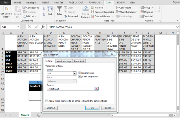
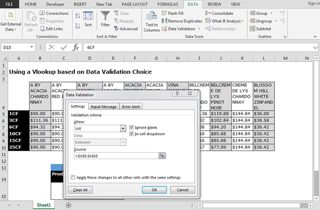

Whenever you will change the product and product code from the drop down list amount will get changed automatically.
The applications/code on this site are distributed as is and without warranties or liability. In no event shall the owner of the copyrights, or the authors of the applications/code be liable for any loss of profit, any problems or any damage resulting from the use or evaluation of the applications/code.


That doesn't work. you cannot select more than one column on a validation data list. Excel gives an error: The list source must be a delimited list, or a reference to a single row, column