
Cascading Dependent Drop Down boxes are a fun and common trick, allowing a second drop down list to change its options based on the selection made in a first drop down box. This is commonly accomplished using the INDIRECT() function.
Another common trick is to use Dynamic Named Range formulas to create named ranges that adjust themselves as you add items to the column. Very useful.
PROBLEM: These two "tricks" do not work together. If you use Dynamic Named Range formulas to create a list of Teams and then use that named range as the source of the DV list in cell A1, you cannot use the INDIRECT(A1) method to select the dependent named range that has the same name as the selected text in A1.
SOLUTION: The workaround then is to not create dynamic named range formulas at all. Instead, you move all the dynamic activity into the Dependent Data Validation "Source" formula.
SETUP:
1.On a Rosters sheet all your lists will reside side-by-side in columns, set them up like so:

2. We create a named range called AnchorCell by clicking on A1 and typing that name into the name box as shown above.
This allows us to create a data validation formula later that will still work on Excel 2003.
3.We create a dynamic named range called Teams by pressing CTRL-F3 and defining the name with the RefersTo formula of:
=OFFSET(Rosters!$A$1, , , 1, COUNTA(Rosters!$1:$1))

This allows you to add new columns (Teams) anytime you want without having to change anything else, it will all keep working and include your new teams as well.
NOTE: No blank columns, this is a reference sheet, keep it tidy.
4. Next, nothing fancy here, we use the named range Teams as the list source for our column A primary data validation on theSelections sheet:

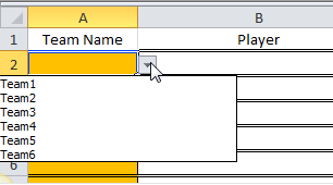
Once applied, it provides a list of the teams from row1 of our Rosters sheet:
5. And here's the magic. The Data Validation list formula in B2 does all the heavy lifting, using OFFSET() and MATCH functions to find the team chosen in column A on row1 of the Rosters sheet, then create a drop down of only the items in that column. In B2, the DV formula would be:
=OFFSET(AnchorCell, 1, MATCH($A2, Teams, 0)-1, COUNTA(OFFSET(AnchorCell, , MATCH($A2, Teams, 0)-1, 50, 1))-1, 1)
You should spend some time reading the help files on offset so the parameters make sense to you:
=OFFSET(reference, rows, columns, [height], [width])
6. Once applied, the secondary list creates itself based on the choice made in the column A cell:

The applications/code on this site are distributed as is and without warranties or liability. In no event shall the owner of the copyrights, or the authors of the applications/code be liable for any loss of profit, any problems or any damage resulting from the use or evaluation of the applications/code.


So smooth, I appreciate this as it is just what I was looking for.
Agree with Alef, a downloadable file would be really nice here!
Put an excel file with all the necessary explanations.