
In this article, we will learn how to use SEARCH function in Microsoft Excel.
The MS-Excel SEARCH function returns the position of the first character of sub-string or search_text in a string. The function does not discriminate between uppercase and lowercase letters while searching. Unlike FIND, SEARCH allows wildcard characters, like question mark (?) and asterisk (*). The question mark (?) matches any single character and the asterisk (*) matches any sequence of character. However, in case we want to find an actual question mark (?) or asterisk (*), we type a tide (~) before the character. If the sub-string is not found within the string, then the function will return #VALUE error. SEARCH function can be used as powerful string method function when combined with MID function.
The function arguments / syntax are: 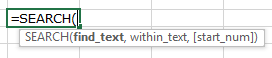 We have dummy data in column A. Column B contains the text which we will search for. And column C has the starting position of the search. And, here in column D, we will enter the SEARCH function.
  1st Example:- In the first example, we will search “AGE” in cell A7.
  Follow the steps given below:-
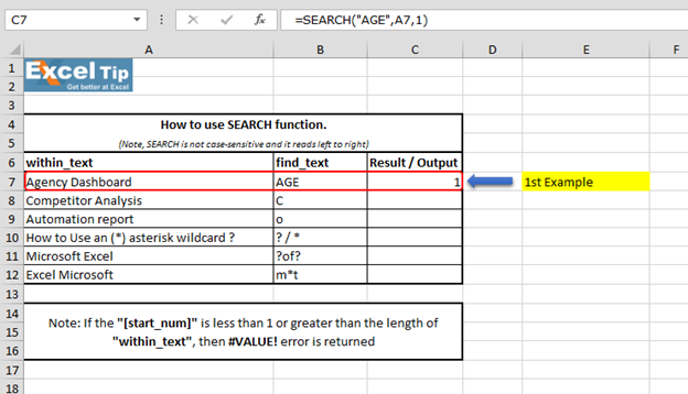 It returns to 1 because “SEARCH” is looking from the first character, and it found AGE beginning from the 1st character. So it gives us 1 here. 2nd Example:- In this example, we will search for “C” and we give the starting number as zero or negative number as the starting position.
 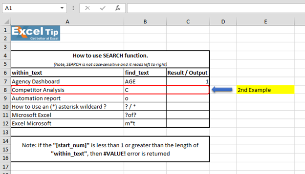 Follow the steps given below:-
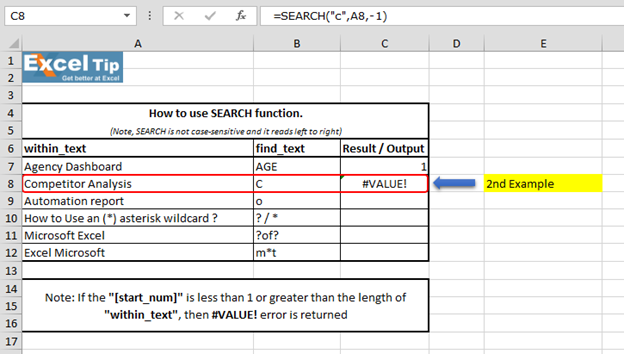 The Function has returned #VALUE error because neither negative nor 0 can be the starting position. 3rd Example:- In this example, we will show you what if we have to find the text which is there multiple times in the string.
 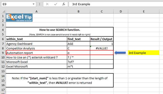 Follow the steps given below:-
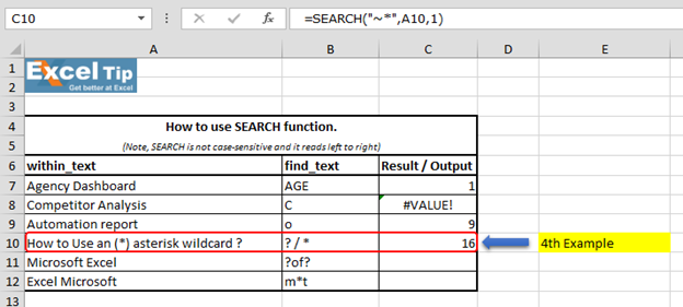
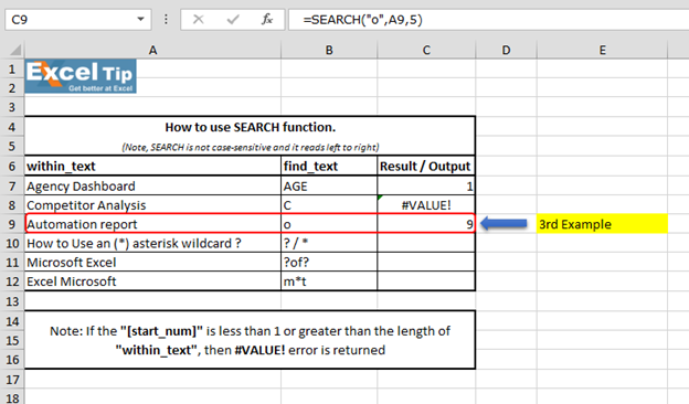 The function has ignored the “o” which is at 4th position and the function returns to 9 as the position. Because it ignored the first “o” and started looking from 5th character onwards. However, it returns the overall position of the string. 4th Example:- In this example, we’ll search for wildcard characters’ position within cell A10.
 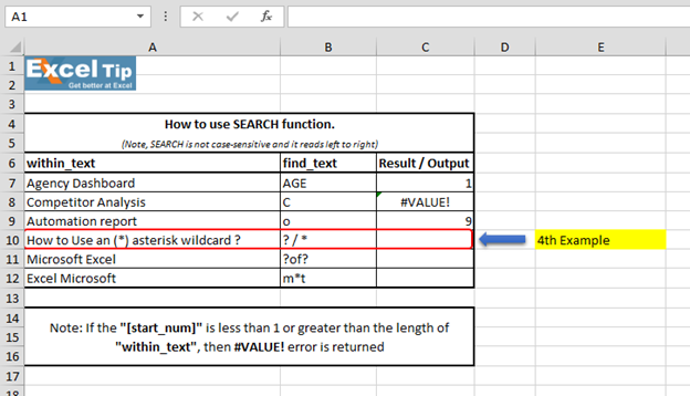 Follow the steps given below:-
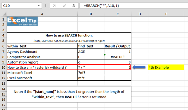 The function has returned 1, because we cannot find any wildcard without using tilde. As we use tilde (~) as a marker to indicate that the next character is a literal, we will insert (~) tilde before (*) asterisk.
 We can also look for question mark:-
 We can see that function gave us “37” as the position of (?) question mark. 5th Example:- In this example, we’ll learn how to enter SEARCH function to search “?of?”.
 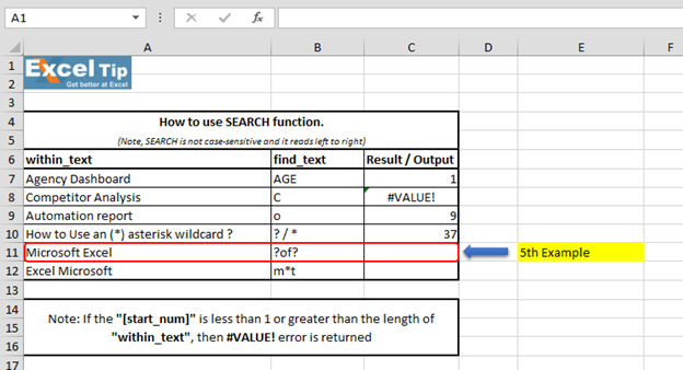 Follow the steps given below:-
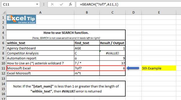 We scan to see that function has returned 6 because it matches “soft” which is present in the mid of “Microsoft Excel” string and hence the value is 6. Note:- (?) question mark wildcard denotes any single character. 6th Example:- In this example, we’ll learn another use of wildcard in SEARCH function.
  Follow the steps given below:-
Note: - In first argument, we tell the function to look for the string which starts with “m” and ends with “t”, and we will put asterisk (*) in between.
 “Microsoft Excel” and it finds there is a string which starts with “M” and ends with “L”. No matter how many characters are there in between and hence it returns 1. Because (*) asterisk wild character matches any sequence of character. So, this is how SEARCH function works in different situation.
 ![]()
Click on the video link for quick reference to the use of SEARCH function. Subscribe to our new channel and keep learning with us! https://www.youtube.com/watch?v=HW0QP1JxeuU
If you liked our blogs, share it with your friends on Facebook. And also you can follow us on Twitter and Facebook. We would love to hear from you, do let us know how we can improve, complement or innovate our work and make it better for you. Write us at info@exceltip.com
The applications/code on this site are distributed as is and without warranties or liability. In no event shall the owner of the copyrights, or the authors of the applications/code be liable for any loss of profit, any problems or any damage resulting from the use or evaluation of the applications/code.


Were is search and delete There used to be a function one could click on and the search box opened, you typed in what you were looking for and it was found. Also you could search and replace. It was all easy noy now it seems I have to work out codes and put them somewhere. why was it changed?
Also I have lost the function to be able to go back on the page and if I had accidentally canceled a word or figure It would put it back for me. I have tried to restore that function and that wont work either.Why do we have to change 2 functions that worked extremely well.
Hi, you can use find in all versions of excel by pressing shortcut CTRL+F. For replacing text, it is CTRL+H. you can still find it on the home tab, in the rightmost corner.
The undo can be done using CTRL+Z.