
In this article, we will learn how to create dynamic drop down list in Microsoft Excel.
As we know Data Validation feature improves the efficiency of data entry in excel and reduces mistakes and typing errors. It is used to restrict the user for the type of data that can be entered in the range. In case of any invalid entry, it shows a message and allows user to enter the data based on specified condition.
But a dynamic drop down list in Excel is a more convenient way of selecting data, without making any changes to the source. In other words, say you are going to update the list frequently which you’ve taken in drop down list. And, you are thinking if you make any changes in the list, you need to modify the data validation every time in order to get the updated drop down list.
But, this is where dynamic drop down comes into the picture, and it is the best option to select data without making any changes in the data validation. It is very similar to the normal data validation. However, when you update the list, the dynamic drop down list changes to accommodate that action, whereas the normal drop down list does not.
So, let’s take an example and understand how we create dynamic drop down list:-
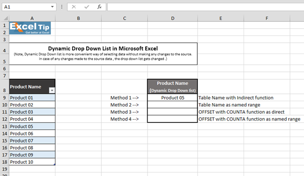
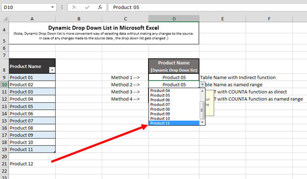
We have a list of products in column A, and, we are going to have the dynamic drop down list of Products in cell D9.
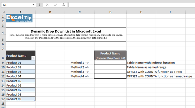
Table Name with Indirect function
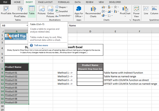
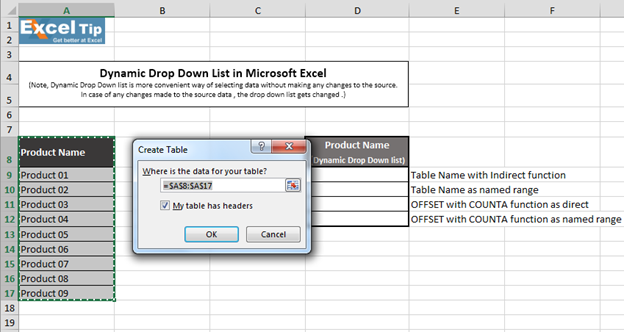
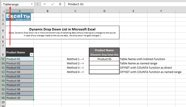
First, we will create table; follow the steps given below:-

Note: - If we add any product or item to the bottom of the list, the table will expand automatically to incorporate the new products or items.
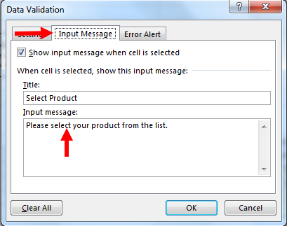
Now we create the dynamic drop down list in cell D9, follow the steps given below:-


Note: - When we click on OK, in Excel, window pops up saying that there is something wrong with the input. That’s because Excel does not accept any self-expanding table directly in the Data Validation.
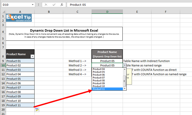
Now add new products, in the product list.
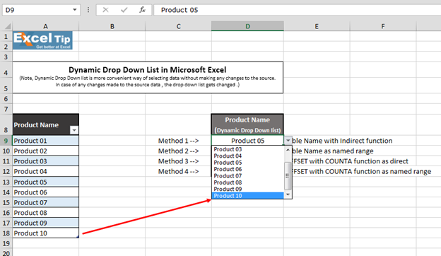
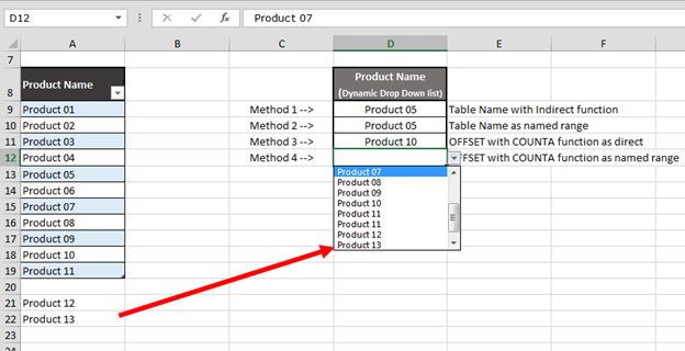
We can see in the above image that new added product is appearing in the drop down list.
2nd Example:-
In this example, we will learn how to give the table name as ranged name
We already have the table name but here we have to define the name of this table to get the dynamic drop list; follow the steps given below:-


Note:- If you do not remember what name you have given to that range, you can press F3 key and a window will pop up to suggest you all the named ranges available.


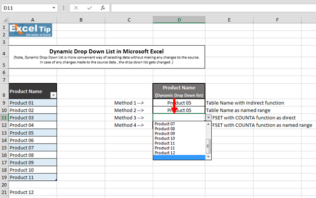
But what happens when we skip one cell after last cell and then add new product or item? You can see, this time the table range has not expanded, and in fact, the newly added product is in general format. So, will it be showing in the drop down list or not? To check that, when we go to cell D10 and check the drop down list, we can see the same old drop down list with no new product. It is because the table range did not find anything after the very last cell and hence the range did not expend.
3rd Example:-
In the next two methods, we’ll learn how we can make our drop down list more dynamic by using OFFSET and COUNTA function.
Follow the steps given below:-
=OFFSET($A$9,0,0,COUNTA($A:$A),1)

Formula Explanation:- We have selected A9, which is the first product in the range, and then we type 0 on the 2nd argument as we don’t want to move row from the starting point; then again 0 in the 3rd argument as here we don’t want any changes in the number of column as well as from the starting point. And then we have entered COUNTA function and have selected entire column A. This argument will check the height in number of rows to return the non-blank count. It will expand the range when any changes are made in the range.
And, the last argument “Width” is an optional argument. It is the width in number of columns. We can either skip it or can type 1 here for now. If we skip, it will, by default, consider the width of the returned range which we supplied in the argument and then we close the parentheses.
4th Example:-
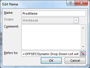
In this example, we will use the function to define the name.
To define the range name, follow the steps given below:-
=OFFSET('Dynamic Drop Down List with DV'!$A$9,0,0,COUNTA('Dynamic Drop Down List with DV'!$A:$A))

So, this is how you can get the dynamic list for any product or item with different methods using data validation. That’s all for now. In the next video of this series, we will explain how to create the dependent drop down list with different methods in Excel.
![]()
Click on the video link for quick reference to the use of it. Subscribe to our new channel and keep learning with us!
If you liked our blogs, share it with your friends on Facebook. And also you can follow us on Twitter and Facebook.
We would love to hear from you, do let us know how we can improve, complement or innovate our work and make it better for you. Write us at info@exceltip.com
The applications/code on this site are distributed as is and without warranties or liability. In no event shall the owner of the copyrights, or the authors of the applications/code be liable for any loss of profit, any problems or any damage resulting from the use or evaluation of the applications/code.


Thanks Thanks Thanks
Hi, is it possible to create the same list but put the list values in a different sheet? How would the formula look then?
Thank You for the tutorial.
Thank you very much for the tips. It really made my workflow much much easier.
This is a great tool! Thank you. So, question: based on a list of task categories using dropdown list 1, can the adjacent cell in that row display different associated drop down lists. For example, if a time sheet had 'Event Support' as the task CATEGORY dependent on the list of task CATEGORY drop list, then in the next column, can you have ONLY a list of task 'ACTIVITIES' associated only with event support. so, only display dropdown list for event support, such as logistics, booth setup, lead acquisition, etc. This would be different for ADVERTISING tasks such as copywriting, layout/design, etc. in this way, the dropdown lists would be shorter and dynamically controlled based on these task categories and task activities.
All your videos are excellent. I want learn more in VBA tips /tricks. Any course is available.