
In this article, we will learn how to sum up top or bottom N values given array of numbers in Excel. If you want to sum top 4, top 5 or top N values in a given range, this article will help do so.
Sum of TOP N values
For this article we will be required to use the SUMPRODUCT function. Now we will make a formula out of these functions. Here we are given a range and we need to top 5 values in range and get the sum of the values.
Generic formula:
range: range of values
Values : numbers separated using the commas like if you wish to find the top 3 values, use { 1 , 2 , 3 }.
Example: Sum Top 5 Values of Range
Let's test this formula via running it on the example shown below.
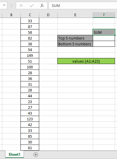
Here we have a range of values from A1:A23.

The range A1:A23 contains values and it is named as values.
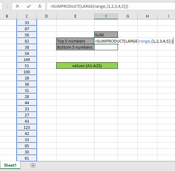
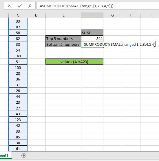
Firstly, we need to find the top five values using the LARGE function and then sum operation be performed over those 5 values. Now we will use the following formula to get the sum of top 5 values.
Use the Formula:
Explanation:
= SUMPRODUCT ( { 149 , 123 , 100 , 87 , 85 } ) )
Here the range is given as the named range. Press Enter to get the SUM of top 5 numbers.
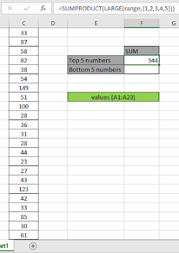
As you can see in the above snapshot, that sum is 544. The sum of the values 149 + 123 + 100 + 87 + 85 = 544.
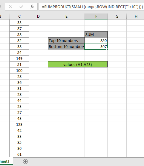
The above process is used to calculate the sum of a few numbers from the top. But to calculate for n (large) number of values in a long range.
Use the formula:
Here we generate sum of top 10 values via getting an array of 1 to 10 { 1 ; 2 ; 3 ; 4 ; 5 ; 6 ; 7 ; 8 ; 9 ; 10 } using the ROW & INDIRECT Excel functions.
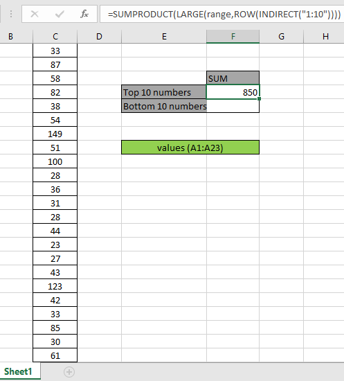
Here we got the sum of the top 10 numbers { 149 ; 123 ; 100 ; 87 ; 85 ; 82 ; 61 ; 58 ; 54 ; 51 }) which results in 850.
How to solve the problem?
Generic formula:
Range: range of values
Values : numbers separated using the commas like if you wish to find the bottom 3 values, use { 1 , 2 , 3 }.
Example:
All of these might be confusing to understand. So, let's test this formula via running it on the example shown below.
Here we have a range of values from A1:A23.
Here is the range that is given using the named range excel tool.
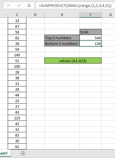
Firstly, we need to find the bottom five values using the SMALL function and then sum operation be performed over those 5 values. Now we will use the following formula to get the sum
Use the Formula:
Explanation:
= SUMPRODUCT ( { 23 , 27 , 28 , 28 , 30 } ) )
Here the range is given as the named range. Press Enter to get the SUM of the bottom 5 numbers.
As you can see in the above snapshot that sum is 136. The sum of the values 23 + 27 + 28 + 28 + 30 = 136.
The above process is used to calculate the sum of a few numbers from the bottom. But to calculate for n (large) number of values in a long range.
Use the formula:
Here we generate sum of bottom 10 values via getting an array of 1 to 10 { 1 ; 2 ; 3 ; 4 ; 5 ; 6 ; 7 ; 8 ; 9 ; 10 } using the ROW & INDIRECT Excel functions.
Here we have the sum of the bottom 10 numbers which will result in 307.
Here are some observational notes shown below.
Notes:
Hope this article about how to Return Sum of top n values or bottom n values in Excel is explanatory. Find more articles on SUMPRODUCT functions here. Please share your query below in the comment box. We will assist you.
Related Articles
How to use the SUMPRODUCT function in Excel: Returns the SUM after multiplication of values in multiple arrays in excel.
SUM if date is between : Returns the SUM of values between given dates or period in excel.
Sum if date is greater than given date: Returns the SUM of values after the given date or period in excel.
2 Ways to Sum by Month in Excel: Returns the SUM of values within a given specific month in excel.
How to Sum Multiple Columns with Condition: Returns the SUM of values across multiple columns having condition in excel
How to use wildcards in excel : Count cells matching phrases using the wildcards in excel
Popular Articles
50 Excel Shortcut to Increase Your Productivity
If with conditional formatting
Convert Inches To Feet and Inches in Excel 2016
Join first and last name in excel
Count cells which match either A or B
The applications/code on this site are distributed as is and without warranties or liability. In no event shall the owner of the copyrights, or the authors of the applications/code be liable for any loss of profit, any problems or any damage resulting from the use or evaluation of the applications/code.


