Formatting a Negative Number with Parentheses in Microsoft Excel
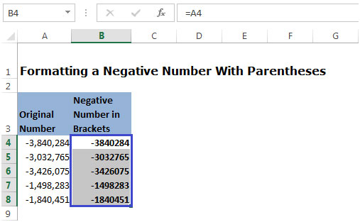
We need to display negative numbers in parentheses to differentiate the positive numbers from the negative numbers.
To display a Negative Number with Parentheses, we can use Excel Custom Formatting.
There are 4 methods by which we can format the Negative Number with Parentheses:
To apply the custom formatting in cell follow below steps:-
Method 1:
We have some negative numbers in column B.
To Format the Negative Numbers in Red Color with brackets:
- Select the cells & right click on the mouse.
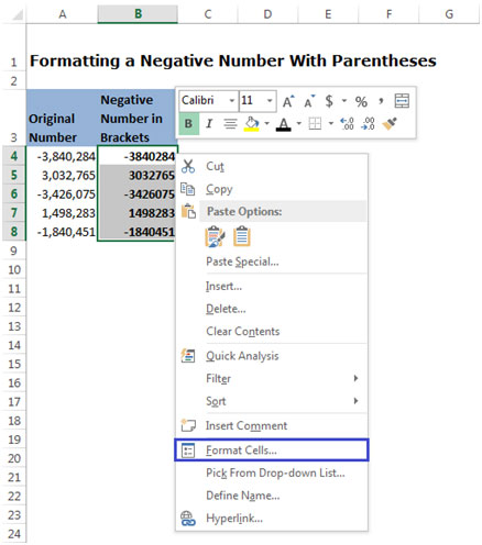
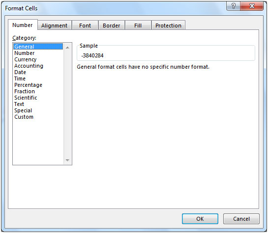
- Click on Format Cells orPress Ctrl+1 on the keyboard to open the Format Cells dialog box.

- Select the Number tab, and from Category, select Number.
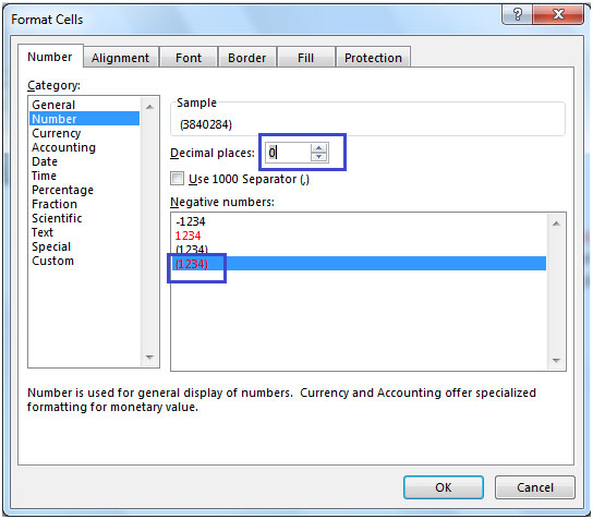
- In the Negative Numbers box, select the last option as highlighted.
- Enter ‘0’ in the Decimal placesbox to avoid decimals.
- Click on Ok.
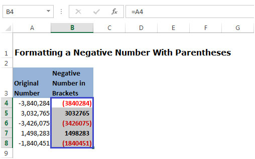
- This is how our data looks after formatting.
Method 2:
To Format the Negative Numbers in Black with brackets:
- Select the cells & right click on the mouse.

- Click on Format Cells orPress Ctrl+1 on the keyboard to open the Format Cells dialog box.

- Select the Number tab, and from Category, select Number.
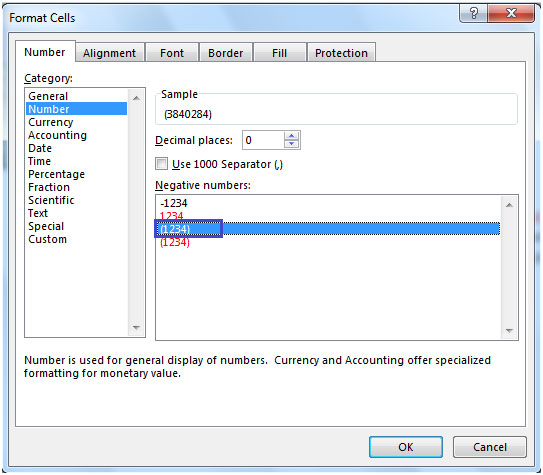
- In the Negative Numbers box, select the 3rd option as highlighted.
- Enter ‘0’ in the Decimal places box to avoid decimals.
- Click on Ok.
- This is how our data looks after formatting.

Method 3:
To Format the Negative Numbers in Red Color with brackets using Custom Formatting:
We have to apply Custom Formatting to the column B as shown in the below screenshot:
- Select the cells & right click on the mouse.

- Click on Format Cells orPress Ctrl+1 on the keyboard to open the Format Cells dialog box.

- Select the Number tab, and from Category, select Custom.

- In the Type box, enter the following Custom Formatting syntax for Red color:
#,##0 ;[Red](#,##0);- ;
- Click on Ok.
- This is how our data looks after formatting.

Method 4:
To Format the Negative Numbers in Black Color with brackets using Custom Formatting -
We have to apply Custom Formatting to the column B as shown in the below screenshot:
- Select the cells & right click on the mouse.

- Click on Format Cells orPress Ctrl+1 on the keyboard to open the Format Cells dialog box.
- Select the Number tab, and from Category, select Custom.

- In the Type box, enter the following Custom Formatting syntax for Black color:
#,##0 ;[Black](#,##0);- ;
or
#,##0;(#,##0);0

- Click on Ok.
- This is how our data looks after formatting.


Quite helpful but, how can I keep this format permanently? Because I dont get this format on any new sheet?