
Para extraer la última palabra del texto en una celda usaremos la función “DERECHA” con la función “HALLAR” y “LARGO” en Microsoft Excel 2010.
DERECHO:Devuelve los últimos caracteres de una cadena de texto en función del número de caracteres especificado.
Sintaxis de la función “DERECHA”: =DERECHA (texto, [num_chars])
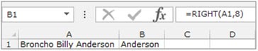
Ejemplo:La celda A1 contiene el texto “Broncho Billy Anderson”
=DERECHA (A1, 8), la función devolverá “Anderson”
HALLAR: La función HALLAR devuelve la posición inicial de una cadena de texto que localiza desde dentro de la cadena de texto.
La sintaxis de la función "BÚSQUEDA": =BUSCAR (texto_buscado,dentro_del_texto,[posición_inicial])
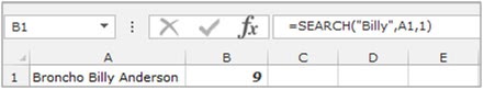
Ejemplo: La celda A2 contiene el texto "Broncho Billy Anderson”
=HALLAR ("Billy", A1, 1), la función devolverá 9
LARGO:Devuelve el número de caracteres de una cadena de texto.
Sintaxis de la función “LARGO”: = LARGO (texto)
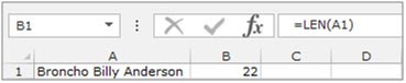
Ejemplo:La celda A1 contiene el texto “Broncho Billy Anderson”
=LARGO (A1), la función devolverá 22
Comprender el proceso de extracción de caracteres del texto mediante fórmulas de texto
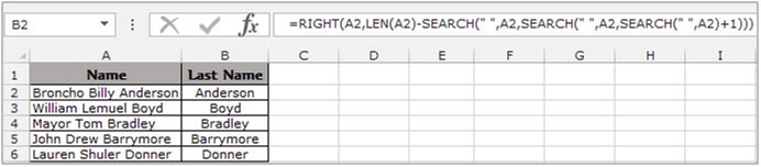
Ejemplo 1: Tenemos una lista de nombres en la columna "A" y tenemos que elegir el apellido de la lista. Usaremos la función "IZQUIERDA" junto con la función "BÚSQUEDA".

Para separar la última palabra de una celda, siga los pasos a continuación:-
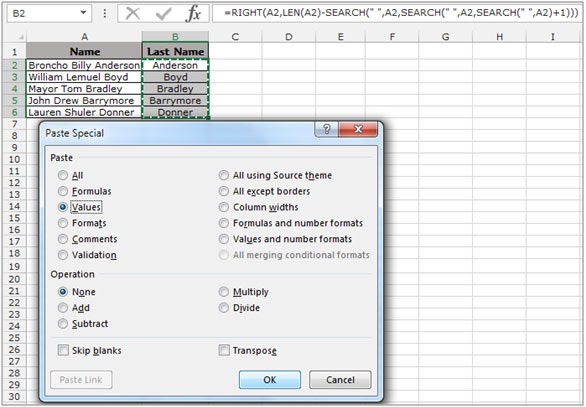
Seleccione la celda B2, escriba la fórmula =DERECHA(A2,LARGO(A2)-HALLAR(" ",A2,HALLAR(" ",A2,HALLAR(" ",A2)+1))) la función devolverá el apellido de la celda A2
Para copiar la fórmula a todas las celdas, presione la tecla "CTRL + C" y seleccione la celda B3 a B6 y presione la tecla "CTRL + V" en su teclado.
Para convertir las fórmulas en valores, seleccione el rango de funciones B2: B6, y "COPY" presionando la tecla "CTRL + C", haga clic con el botón derecho del mouse para seleccionar "Pegar especial".
Aparecerá el cuadro de diálogo Pegar especial. Haga clic en "Valores" y luego haga clic en Aceptar para convertir la fórmula en valores.
Así es como podemos extraer la última palabra de una celda en otra celda.
The applications/code on this site are distributed as is and without warranties or liability. In no event shall the owner of the copyrights, or the authors of the applications/code be liable for any loss of profit, any problems or any damage resulting from the use or evaluation of the applications/code.


