

Microsoft Excel tiene tantas capacidades increíbles que no se perciben instantáneamente. Las teclas de acceso directo de Excel son más útiles y utilizables para ahorrar tiempo.
Las teclas de método abreviado ayudan a proporcionar un método más fácil y, por lo general, más rápido de dirigir y finalizar comandos en Microsoft Excel. En general, preferimos usar los atajos, ya que es asombroso cuánto tiempo podemos ahorrar si no usamos los clics del mouse. Los atajos de teclado en Excel se acceden comúnmente usando ALT, Ctrl, Shift, tecla de función y tecla de ventana.
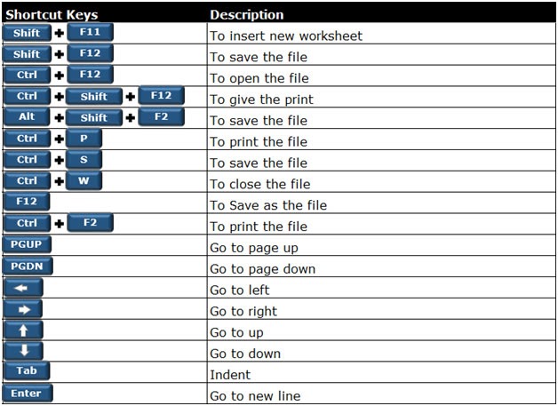
Nos gustó mucho que Windows nos brinda múltiples formas de realizar la tarea en Excel, digamos que queremos guardar un archivo, o podemos presionar la tecla "Ctrl + S" o "Shift + F11".
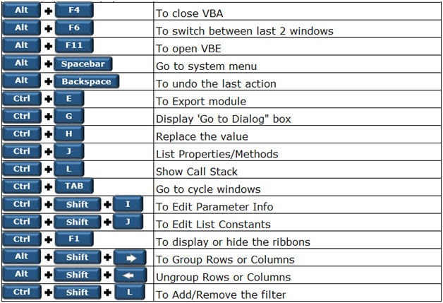
A continuación se muestran los increíbles atajos para la categoría de Excel, en los que encontrará los atajos de fórmulas de Excel, los atajos de copiar y pegar de Excel, los atajos de teclado de Excel para insertar una fila, los atajos de teclado de Excel para seleccionar la fila, los atajos de teclado para VBA y las teclas de acceso rápido de Excel (agregue más Alt atajos a Excel).
Atajos de teclado para el cuadro de diálogo: -

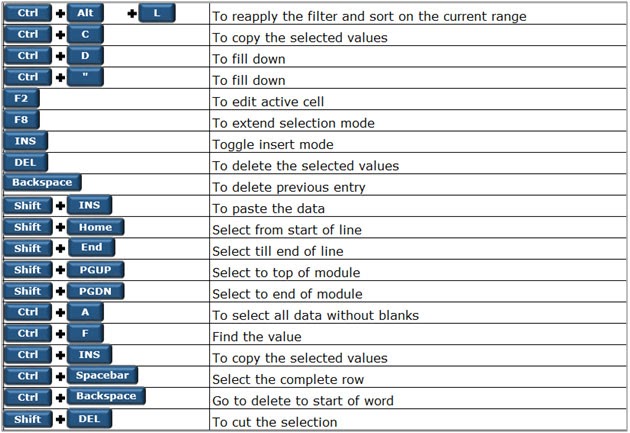
Ingresar atajos de datos: -

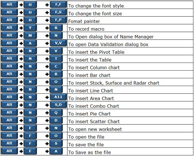
Comandos de archivo: -
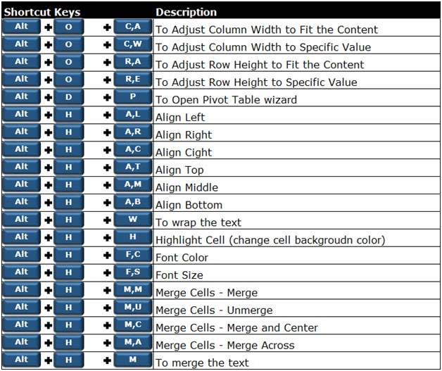
Atajos de teclado para formato: -


Métodos abreviados de fórmulas: -

Atajos de teclado generales: -

Teclas de acceso rápido importantes: -
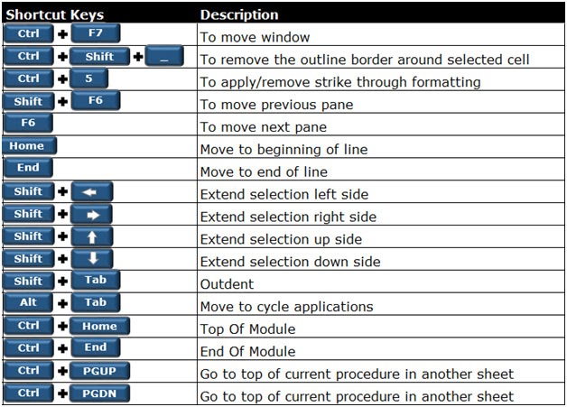
Accesos directos para navegar: -


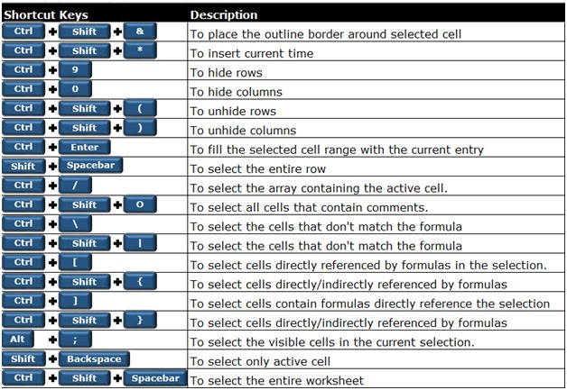
Atajos de teclado para seleccionar filas / columna / celda: -
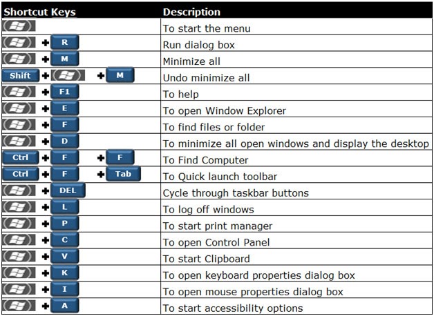
Teclas de atajo de ventana: -
Teclas de método abreviado del libro de trabajo: -

The applications/code on this site are distributed as is and without warranties or liability. In no event shall the owner of the copyrights, or the authors of the applications/code be liable for any loss of profit, any problems or any damage resulting from the use or evaluation of the applications/code.


