
Muchas veces, queremos calcular algunos valores por mes. Como por ejemplo, cuánto se vendió en un mes en particular. Bueno, esto se puede hacer fácilmente usando tablas pivotantes, pero si se trata de tener un informe dinámico, podemos usar una fórmula de SUMPRODUCTOS o SUMAS para sumar por mes.
Comencemos con la solución SUMPRODUCTO.
Aquí está la fórmula genérica para obtener la suma por mes en Excel
| =SUMPRODUCTO(suma_range,--( TEXT(fecha_range, "MMM")=month_text)) |
Suma_range : Es el rango que quieres sumar por mes.
Rango_de_fechas : Es el rango de fechas que buscarás por meses.
Texto_mes: Es el mes en formato de texto del que quieres sumar valores.
Ahora veamos un ejemplo:
Ejemplo: Sumar valores por mes en Excel
Aquí tenemos algún valor asociado a las fechas. Estas fechas son de enero, febrero y marzo del año 2019.

Como pueden ver en la imagen de arriba, todas las fechas son del año 2019. Ahora sólo tenemos que sumar los valores en E2:G2 por meses en E1:G1.
Ahora para sumar valores según los meses escriban esta fórmula en E2:
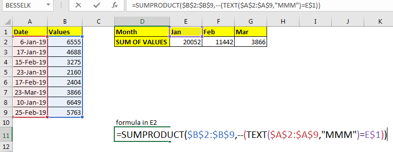
| =SUMPRODUCTO(B2:B9,--(TEXTO(A2:A9, "MMM")=E1)) |
Si quieres copiarlo en celdas adyacentes, entonces usa referencias absolutas o rangos nombrados como en la imagen.
Esto nos da la suma exacta de cada mes.
¿Cómo funciona?
Empezando desde el interior, veamos la parte del texto (A2:A9, "MMM"). Aquí la función TEXTO extrae el mes de cada fecha en el rango A2:A9 en formato de texto en una matriz. Traduciendo a la fórmula a =SUMPRODUCTO(B2:B9,--({"Jan"; "Jan"; "Feb"; "Jan"; "Feb"; "Mar"; "Jan"; "Feb"}=E1))
A continuación, TEXT(A2:A9, "MMM")=E1: Aquí cada mes en la matriz se compara con el texto en E1. Como E1 contiene "Jan", cada "Jan" en la matriz se convierte en VERDADERO y el resto en FALSO. Esto traduce la fórmula a
| =SUMPRODUCTO($B$2:$B$9,--{Verdadero;Verdadero;Falso;Verdadero;Falso;Falso;Verdadero;Falso}) |
Siguiente --(TEXTO(A2:A9, "MMM")=E1), convierte FALSO VERDADERO en valores binarios 1 y 0. La fórmula se traduce a =SUPREMO($B$2:$B$9,{1;1;0;1;0;0;1;0}).
Finalmente SUMAPRODUCTO($B$2:$B$9,{1;1;0;1;0;0;1;0}): la función SUMAPRODUCTO multiplica los valores correspondientes en $B$2:$B$9 al conjunto {1;1;0;1;0;0;1;0} y los suma. Por lo tanto, obtenemos la suma por valor como 20052 en E1.
SUMAR LOS MESES DE DIFERENTE AÑO
En el ejemplo anterior, todas las fechas eran del mismo año. ¿Y si eran de años diferentes? La fórmula anterior sumará los valores por mes, independientemente del año. Por ejemplo, se sumarán enero de 2018 y enero de 2019, si usamos la fórmula anterior. Lo cual es incorrecto en la mayoría de los casos.
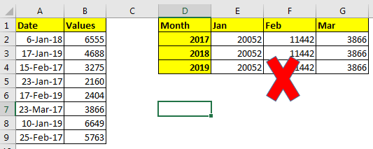
Esto sucederá porque no tenemos ningún criterio para el año en el ejemplo anterior. Si añadimos el criterio del año también, funcionará.
La fórmula genérica para obtener la suma por mes y año en Excel
| =SUMPRODUCTO(suma_range,--( TEXT(fecha_range, "MMM")=month_text),--( TEXT(fecha_range, "yyyy")=TEXT(year,0)) |
Aquí, hemos añadido un criterio más que comprueba el año. Todo lo demás es igual.
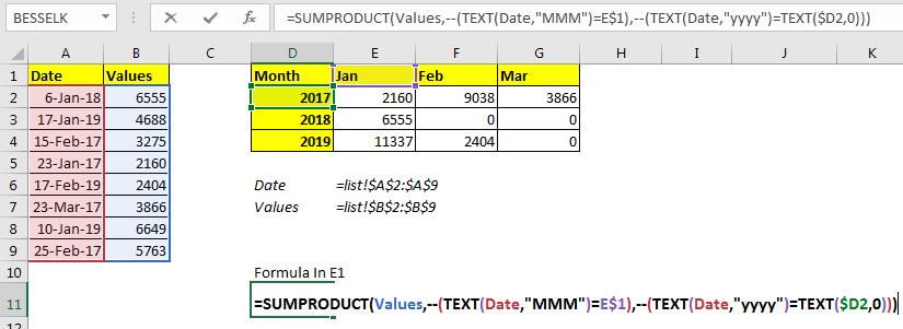
Resolvamos el ejemplo anterior, escribamos esta fórmula en la celda E1 para obtener la suma de Jan en el año 2017.
| =SUMPRODUCTO(B2:B9,--(TEXTO(A2:A9, "MMM")=E1),--(TEXTO(A2:A9, "yyyy")=TEXTO(D2,0)) |
Antes de copiar en las celdas de abajo utilice rangos nombrados o referencias absolutas. En la imagen, he usado rangos con nombre para copiar en las celdas adyacentes.

Ahora podemos ver la suma de valor por meses y años también.
¿Cómo funciona?
La primera parte de la fórmula es la misma del ejemplo anterior. Entendamos la parte adicional que añade el criterio del año.
--(TEXTO(A2:A9, "yyyy")=TEXTO(D2,0)): TEXTO(A2:A9, "yyyy") convierte la fecha en A2:A9 como años en formato de texto en una matriz. {"2018";"2019";"2017";"2017";"2019";"2017";"2019";"2017"}.
La mayoría de las veces, el año se escribe en formato numérico. Para comparar un número con el texto que nosotros, he convertido el año en texto usando TEXT(D2,0). A continuación comparamos este año de texto con una matriz de años como TEXT(A2:A9, "yyyy")=TEXT(D2,0). Esto devuelve una matriz de verdadero-falso {FALSO;FALSO;VERDADERO;VERDADERO;FALSO;VERDADERO}. A continuación convertimos el verdadero falso en un número usando el operador --. Esto nos da {0;0;1;1;0;1;0;1}.
Así que finalmente la fórmula será traducida a =SUPREMO(B2:B9,{1;1;0;1;0;0;1;0},{0;0;1;1;0;1;0;1}). Donde la primera matriz son los valores. El siguiente es el mes y el tercero es el año. Finalmente obtenemos nuestra suma de valores como 2160.
Usando la función SUMAR.SI.CONJUNTO para sumar por mes
Fórmula genérica
| =SUMIFS(sum_range,date_range,">=" & startdate, date_range,"<=" & EOMONTH(start_date,0)) |
Aquí, Sum_range : Es el rango que quieres sumar por mes.
Rango_de_fechas : Es el rango de fechas que buscarás por meses.
Fecha de inicio : Es la fecha de inicio a partir de la cual quieres hacer la suma. Para este ejemplo, será el 1er del mes dado.
Ejemplo: Sumar valores por mes en Excel
Aquí tenemos algún valor asociado a las fechas. Estas fechas son de enero, febrero y marzo del año 2019.
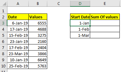
Sólo tenemos que sumar estos valores por ese mes. Ahora era fácil si teníamos meses y años por separado. Pero no es así. No podemos usar ninguna columna de ayuda aquí.
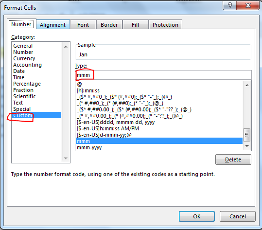
Así que para preparar el informe, he preparado un formato de informe que contiene el mes y la suma de los valores. En la columna del mes, tengo la fecha de inicio del mes. Para ver sólo el mes, seleccione la fecha de inicio y pulse CTRL+1.
En el formato personalizado, escriba "mmm".

Ahora tenemos nuestros datos listos. Sumemos los valores por mes.
Escriba esta fórmula en E3 para sumar por mes.
| =SUMIFS(B3:B10,A3:A10,">="&D3,A3:A10,"<="&EOMONTH(D3,0)) |
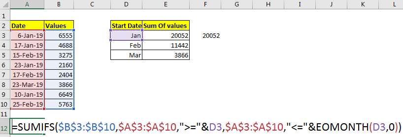
Utilice referencias absolutas o rangos nombrados antes de copiar la fórmula.
Así que, finalmente tenemos el resultado.
Entonces, ¿cómo funciona?
Como sabemos que la función SUMAR.SI.CONJUNTO puede sumar valores en múltiples criterios.
En el ejemplo anterior, el primer criterio es la suma de todos los valores en B3:B10 donde, la fecha en A3:A10 es mayor o igual a la fecha en D3. D3 contiene 1-Ene. Esto se traduce también.
| =SUMIFS(B3:B10,A3:A10,">="& “1-jan-2019” ,A3:A10,"<="EOMONTH(D3,0)) |
El siguiente criterio es la suma sólo si la fecha en A3:A10 es menor o igual que EOMONTH(D3,0). La función EOMONTH sólo devuelve el número de serie de la última fecha del mes proporcionada. Finalmente la fórmula también se traduce.
| =SUMIFS(B3:B10,A3:A10,">=1-jan-2019” ,A3:A10,"<=31-jan-2019”) |
Por lo tanto, obtenemos la suma por mes en Excel.
La ventaja de este método es que se puede ajustar la fecha de inicio para sumar los valores.
Si sus fechas tienen años diferentes, es mejor usar tablas pivotantes. Las tablas pivotantes pueden ayudarte a segregar los datos en formato anual, trimestral y mensual es fácil.
Así que sí, así es como puedes sumar los valores por mes. Ambas formas tienen sus propias especialidades. Elige la forma que más te guste.
Si tienes alguna duda sobre este artículo o cualquier otra consulta relacionada con Excel y VBA, la sección de comentarios está abierta para ti.
The applications/code on this site are distributed as is and without warranties or liability. In no event shall the owner of the copyrights, or the authors of the applications/code be liable for any loss of profit, any problems or any damage resulting from the use or evaluation of the applications/code.


