
The UPPER function in excel is used to capitalize all letters of a string. In this article, we will explore how you can use UPPER function to do some really important tasks. Let’s get started.
Excel UPPER Function Syntax
Text: it is the text or string that you want to capitalize.
Excel Upper Example 1:
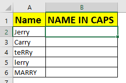
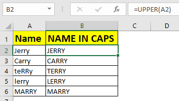
In this example, we just want to get upper case input from the user. So in a column, a user will enter their name. It can be in lower, upper, proper or irregular styled text. In Column B, we just want the upper case text of the A column.
Write the below formula in B1 and copy down.
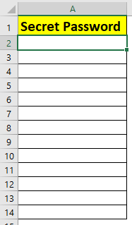
Excel UPPER Example 2: Getting Only Upper Case Inputs
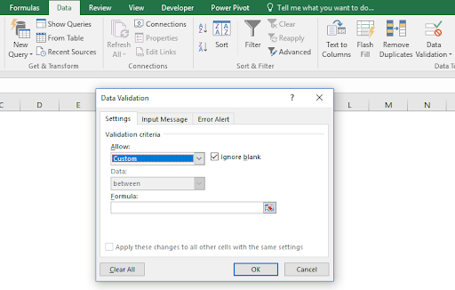
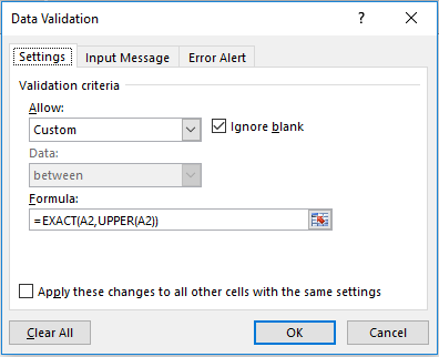
Many times you would want the user to input only UPPER case letters. In this case, we would put a data validation in excel.
Here, we have a column called verification code. Let’s say you have some guest invited in secret party. Now you have cent they the secret code. They will enter their secret code in excel column. The trick is, each code should be in UPPER case. So if any user puts a non upper input, it will show error.
Now try to enter any text that is non-upper case.
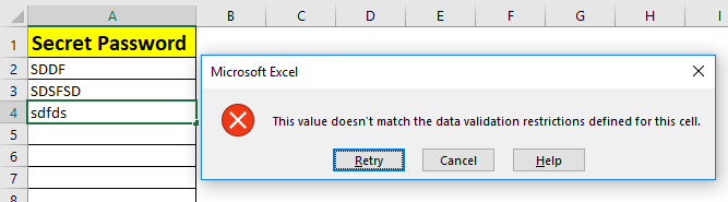
It will not accept the input.
How it Works
Here, we compare text entered in cell, with upper case of that text using EXACT function. If they don’t match, excel shows invalid input prompt.
So yeah guys, this how you use UPPER function in excel. Let me know if you have any doubt about this function of excel in the comments section below.
Related Articles:
How to Use LOWER function in Excel
How to Use PROPER function in Excel
How to use EXACT Function in Excel
How to do Case Sensitive Lookup in Excel
Popular Articles:
50 Excel Shortcuts to Increase Your Productivity
How to use the VLOOKUP Function in Excel
The applications/code on this site are distributed as is and without warranties or liability. In no event shall the owner of the copyrights, or the authors of the applications/code be liable for any loss of profit, any problems or any damage resulting from the use or evaluation of the applications/code.


it's very useful.
thanks.
"1 if u want column a from 1-10 then copy cell a1 to b1
2 apply upper formula
3 copy formula in b1 to all rows till b10
4 copy b1-b10 and paste-special--> values at position a1
UPPPER CASE FOR COLUMNS
WBl77 Posted on: 31-12-1969
YOU CAN USE THE UPPER FORMULA ON THE FIRST CELL, AND THEN USE THE SMALL + AT THE BOTTOM OF THE CELL TO GO TO THE BOTTOM OF THE COLUMN. THIS WILL REPLACE ALL OF THE VALUES IN THE FORMULA WITH THE CELL NUMBERS FOR THE RANGE YOU HIGHLIGHT. THEN JUST REPEAT FOR EACH COLUMN"
"You can down load ASAP Utilites which has a converter to all selected cells.
http://www.asap-utilities.com/"
I could not get this to work at all. If any one know a way to convert entire columns to upper case, it would save me a lot of time. thanks.
This tip works when converting a single cell, but I cannot find how to convert an entire worksheet like I can in WORD. I tried entering =UPPER(A1:J254) but it did not work. My data list is a chart of names and addresses with columns of figures and I want to change the text parts to upper case.
when I enter this formula I get a circular reference. How do I get rid of that. I also would like to convert entire columns at one time. Anyone got the solution.
This tip works when converting a single cell, but I cannot find how to convert an entire worksheet like I can in WORD. I tried entering =UPPER(A1:J254) but it did not work. My data list is a chart of names and addresses with columns of figures and I want to change the text parts to upper case.