
In this article we will learn how to calculate the quarter number for Fiscal Year and Calendar Year in Microsoft Excel.
To calculate quarter in Excel you can use the formula of “INT”, “MONTH”, “MOD” and “CEILING” function.
INT function is used to return the whole number without decimals. This is better than changing the number of decimal places displayed, which would risk some numbers being rounded up and thus giving an incorrect result.
MOD function is used to returns the remainder after a number is divided by a divisor.
MONTH function is used to return the month in numbers.
CEILING function is used to roundup the number to the nearest multiple of a specified value.
Let’s take an example and understand how to calculate the quarter number.
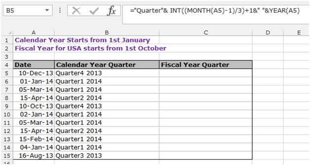
We have a table of dates, in which we want to return the quarter according to the calendar year and fiscal year.
To calculate excel date quarter for a calendar year:-
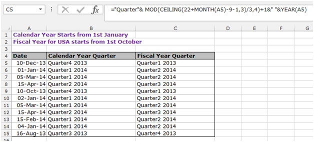
To calculate the quarter number for a fiscal year ending in September:
This function is useful when you have to do certain analysis based on quarters and compare the data of one quarter with another.
Also, you can choose whether you need the quarter as per the financial year or as per the fiscal year and use the appropriate formula to give you the right quarter numbers for your data.
![]()
If you liked our blogs, share it with your friends on Facebook. And also you can follow us on Twitter and Facebook.
We would love to hear from you, do let us know how we can improve, complement or innovate our work and make it better for you. Write us at info@exceltip.com
The applications/code on this site are distributed as is and without warranties or liability. In no event shall the owner of the copyrights, or the authors of the applications/code be liable for any loss of profit, any problems or any damage resulting from the use or evaluation of the applications/code.


Except the fiscal year is incorrect .... October to December 2014 would be Q1 2015, not 2014. The USA FY 2016 is from Oct 2015 - Sep 2016.
This requires a fairly simple mod although it make the formula far more challenging to read.
If your date is in J2, as mine is...
=IF(MOD(CEILING(22+MONTH(J2)-9-1,3)/3,4)+1>1,"FFY"&YEAR(J2)&"-"&MOD(CEILING(22+MONTH(J2)-9-1,3)/3,4)+1,"FFY"&YEAR(J2)+1&"-"&MOD(CEILING(22+MONTH(J2)-9-1,3)/3,4)+1)
This checks to see if the quarter is > 1 and if so keeps the current year. If not it adds a year to the current year.
for Quarter Finding, if C2 is my date:
1. =(TRUNC((MONTH(C2)-1)/3))+1
2. =(INT((MONTH(C2)-1)/3))+1
3. =INT(CEILING(MONTH(C2),3)/3)
4. =INT((CEILING(MONTH(C2),3)+1)/3)
5. =LOOKUP(MONTH(C2),{1,4,7,10},{1,2,3,4})
6. =ROUNDUP(MONTH(C2)/3,0)
7. =HLOOKUP(MONTH(C2),{1,2,3,4,5,6,7,8,9,10,11,12;1,1,1,2,2,2,3,3,3,4,4,4},2)
8. =CHOOSE(MONTH(C2),1,1,1,2,2,2,3,3,3,4,4,4)
=INT(([@Month]-1)/3)+1
=ROUNDUP([@Month]/3,0)
=CHOOSE([@Month],1,1,1,2,2,2,3,3,3,4,4,4) <- Nice for fiscal quarters
Hi Bernardo,
Please try below mentioned formula:-
="Quarter"& MOD(CEILING(22+MONTH(A5)-10-1,3)/3,4)+1&" "&YEAR(A5)
Thanks
Nisha
Hello Maitrey,
My company beguin the fiscal year on 01-11-2014
how can i foun the quarter for any date.
Thnaks
Bernardo
Simple Solution is to use the lookup function:
for example if you want the quarter for 28/02/2014 in MS Excel simply use the function below:
="Q"&LOOKUP(MONTH("28/2/2014"),{1,4,7,10},{1,2,3,4})
"I also use lookup function, but I do not create extra table with month and quarter numbers. I write it directly into formula, for example:
=HLOOKUP(A1,{1,2,3,4,5,6,7,8,9,10,11,12;1,1,1,2,2,2,3,3,3,4,4,4},2)
where A1 is month number
J."
I'm sure the tip shown works but I have used a cheap & dirty vlookup on a table that I create. The table has 2 columns, column 1 has numbers 1-12 which represent months, column 2 reads: 1 1 1 2 2 2 3 3 3 4 4 4 I just vlookup the month in whatever source date I'm using to the month in my lookup table and return the column 2 value. Works for me !! J.
for Quarter Finding, if C2 is my date:
1. =(TRUNC((MONTH(C2)-1)/3))+1
2. =(INT((MONTH(C2)-1)/3))+1
3. =INT(CEILING(MONTH(C2),3)/3)
4. =INT((CEILING(MONTH(C2),3)+1)/3)
5. =LOOKUP(MONTH(C2),{1,4,7,10},{1,2,3,4})
6. =ROUNDUP(MONTH(J2)/3,0)
7. =HLOOKUP(MONTH(J2),{1,2,3,4,5,6,7,8,9,10,11,12;1,1,1,2,2,2,3,3,3,4,4,4},2)
8. =CHOOSE(MONTH(J2),1,1,1,2,2,2,3,3,3,4,4,4)