
In this article, we will learn Advanced Conditional Formatting Tricks in Excel.
Scenario:
Microsoft Excel is having so many unbelievable capabilities that are not instantly perceived. In which Conditional Formatting is one of the options. Conditional Formatting is the tool that is used to format the cell or a range in the specific condition. We can use this option on the value of the cell or value of formula, it means if you have formula in cell then we can specify the value in “Conditional Formatting” of if we have value in the range then we can use Conditional Formatting by describing the formula to highlight the values.
There are a lot of ways to use “Conditional Formatting” in our data. We can use it to show the numbers in increasing and decreasing order, to specific Value, to specific numbers, to specific date etc. Also we can highlight the cells by filling the color in cell, by change the font color, by using the data bars, color scales, icon sets.
Learning more Conditional formatting in Excel
Below are some problems which we handle in day to day problems to highlight cells having condition using Conditional formatting in excel.
For this you need some basic steps. Conditional formatting format cells only if the given condition is True. So you can use any formula which returns True or False. Just try the formula in some cell before using it in the conditional formatting formula box because cell results can check for errors if any.
Example :
All of these might be confusing to understand. Let's understand how to use the function using an example. Here we have some tricks to explain one by one.
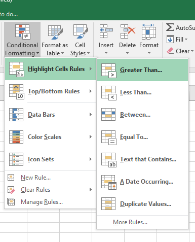
Highlight a cell dependent on another cell
In Conditional formatting, there needs to be condition. Here condition is if some cell satisfies a condition, then format another cell. In short, formatting one cell depending on another cell. Here we have data, and we need to format IDs if the nights spent is greater than or equal to 5. Follow the steps.
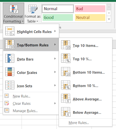
First thing first, If we are formatting IDs, we will select only the ID column. This step is important. Now go to Conditional formatting > New rule. Reference from the below snapshot.
This will open up a new Formatting rule dialog box. Select Use a formula to which cells to determine from the Select a rule type and
Use the formula:
| =E2>=5 |
You need to type this because selecting reference and editing it will be more difficult.
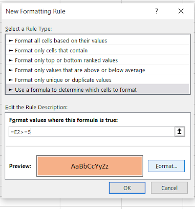
Select the format from the format box. You can format font style, font size, font colour, cell style or cell background colour. Here we just selected the background color as Orange. And the same can be viewed and confirmed in Preview. Now Click OK to get the formatted result.
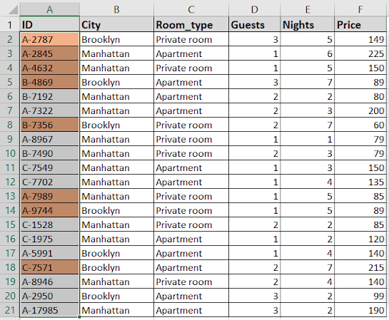
As you can see from the above snapshot, the corresponding ID where nights greater than or equal to 5 are formatted.
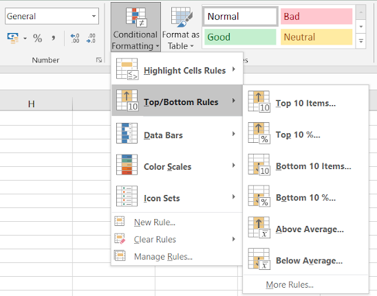
Formatting based on Date column
Dates are interpreted as serial numbers in excel. So just treat the date values as numbers. But it's not easy to remember all serial numbers for all the date values. So use cell reference to pick a date from another cell or use the DATE function providing year, month and date value. Let's learn through as explained below.
Follow the steps here. Select the date values as list and Go to Conditional formatting > New rule.
This will open a Formatting rule box.
Here we need to format date cells which lay between the two given dates. So First we fill any two cells with the given dates in I5 and I6. Just select Use a formula to determine which cells to format. And enter the formula.
Use the formula:
| =AND(G2>$I$5,G2<$I$6) |
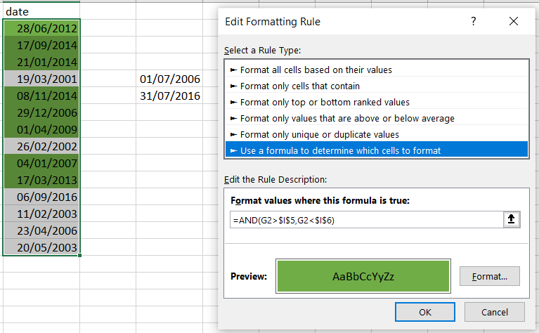
In the above image. AND function checks both conditions and returns True only if both are True or else False. Conditional formats values based on formula returning True and False.
Hide Zeros using Conditional formatting
This is the way to make zero (0) invisible with the background data, so zero values in the table don't get printed. Generally the excel cell background is White. So you can either change the background color to the same color of font or vice-versa. Here we select the data and Go to Conditional Formatting > Highlight Cells Rules > Equal To.
The applications/code on this site are distributed as is and without warranties or liability. In no event shall the owner of the copyrights, or the authors of the applications/code be liable for any loss of profit, any problems or any damage resulting from the use or evaluation of the applications/code.


Hi
Looking for something like this