How to use the PV and FV function in Excel

In this article, we will learn How to use the PV and FV function in Excel.

What is present value and future value ?

Amount is volatile and changes its value as per time and type of investment. For example, banks loan you money on some interest rate and when they provide interest on the deposited amount. So to measure your present value to future or future to present value. Use the PV function to get the present value as per predicted future value. Use the FV function to get the future value as per given present value. Let's learn about the Syntax of PV function and illustrate an example on the same.

PV Function in Excel

PV function returns the present value of the fixed amount paid over a period of time at a constant interest rate.

Syntax:

rate: Interest rate per period

nper: total no. of payment period.

pmt: amount paid each period.

fv - [optional] The present value of future payments must be entered as a negative number.

type - [optional] When payments are due. Default is 0.

FV function in Excel

FV function returns the future value of the present  amount having interest rate over a period.

Syntax:

rate: Interest rate per period

nper: total no. of payment period.

pmt: amount paid each period.

pv - [optional] The present value of future payments must be entered as a negative number.

type - [optional] When payments are due. Default is 0.

Present value (PV function) and Future value (FV function) are both returns amount opposite to each other. The PV function takes argument as future to return the present value whereas the FV function takes present value as argument and returns the future value for the data

Example :

All of these might be confusing to understand. Let's understand how to use the function using an example. Here we first calculate the future value using the present value and vice versa.

Here we have the amount of $100,000 as present value considered over a period of year (12 months) at a rate of 6.5%.

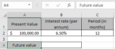
And we need to find the new amount for the data after one year. We will use the FV function formula to get that new amount or future value.

Use the Formula:

Explanation: 

B2/12 : rate is divided by 12 as we are calculating interest for monthly periods.

C2 : the total time period (in months)

0 : no amount paid or received between the total period

-A2 : amount is in negative so as to get the future value amount in positive.

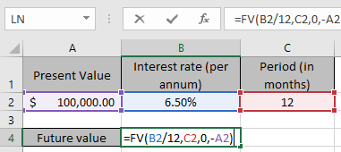
Here argument to the function are given as cell reference.

Press Enter to get the result.

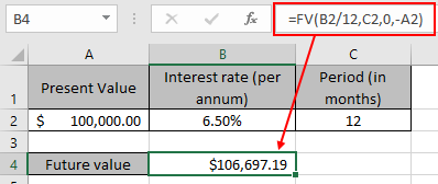
This function returns a value of the amount $106,697.19 as future value for the dataset.

Now consider the same future value for the new data set.

Here we have the amount of $106.697.19 as the future value considered over a period of year (12 months) at a rate of 6.5%.

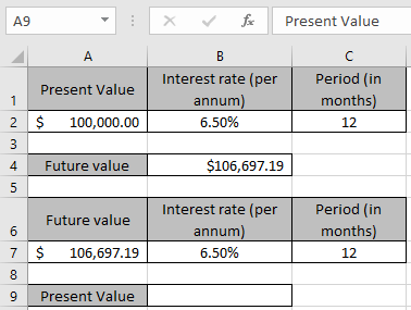
And we need to find the present amount for the data before the year. We will use the FV function formula to get that present value amount.

Use the Formula:

Explanation: 

B7/12 : rate is divided by 12 as we are calculating interest for monthly periods.

C7 : the total time period (in months)

0 : no amount paid or received between the total period

-A7 : amount is in negative so as to get the present value amount in positive.

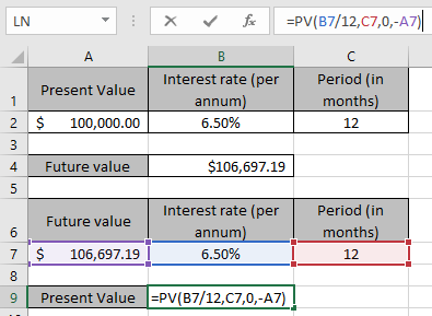
Here argument to the function are given as cell reference.

Press Enter to get the result.

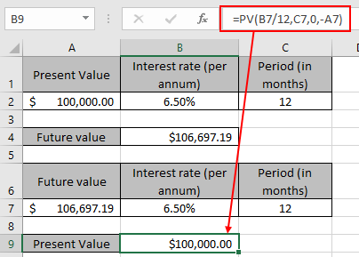
This function returns a value of the amount $100,000 as the same present value for the dataset. As you can see the both functions

Here are all the observational notes using the PV and FV function function in Excel
Notes :

1. Be careful using the rate and npr argument in FV function. If monthly payments on a six-year loan at 15 percent annual interest, use 15%/12 for rate and 6*12 for nper. If made an annual payment on the same loan, use 15% for rate and 6 for nper.
2. When working with Excel currency values. The amount represented in negative such as deposits to savings. dividends and checks to be input as positive numbers.
3. Excel stores dates as serial numbers and is used in calculation by the function. So it’s recommended to use dates as cell reference instead of giving direct argument to the function. Check the date values if the function returns #VALUE! Error.

Hope this article about How to use the PV function in Excel is explanatory. Find more articles on financial values and related Excel formulas here. If you liked our blogs, share it with your friends on Facebook. And also you can follow us on Twitter and Facebook. We would love to hear from you, do let us know how we can improve, complement or innovate our work and make it better for you. Write to us at info@exceltip.com.

Related Articles :

How to use the MIRR function in excel : returns the Modified interest rate of return for the financial data having Investment, finance rate & reinvestment_rate using the MIRR function in Excel.

How to use the XIRR function in excel : returns the Interest rate of return for irregular interval using the XIRR function in Excel

Excel PV vs FV function : find Present Value using PV function and future value using FV function in Excel.

How to use the RECEIVED function in excel : calculates the amount which is received at maturity for a bond with an initial investment (security) and a discount rate, there are no periodic interest payments using the RECEIVED function in excel.

How to use the NPER function in excel : NPER function to calculate periods on payments in Excel.

How to use the PRICE function in excel : returns the price per $100 face value of a security that pays periodic interest using the PRICE function in Excel.

Popular Articles :

How to use the IF Function in Excel : The IF statement in Excel checks the condition and returns a specific value if the condition is TRUE or returns another specific value if FALSE.

How to use the VLOOKUP Function in Excel : This is one of the most used and popular functions of excel that is used to lookup value from different ranges and sheets.

How to use the SUMIF Function in Excel : This is another dashboard essential function. This helps you sum up values on specific conditions.

How to use the COUNTIF Function in Excel : Count values with conditions using this amazing function. You don't need to filter your data to count specific values. Countif function is essential to prepare your dashboard.