
In this article, we will learn How to Sum Stock Lists in Excel.
Stock lists in Excel
Stocks are bought daily by many people. Handling and keeping its data is very crucial as it holds the total profit or loss. The profit or loss of any stock can be called as square off or spread. Each stock is bought on two basis Quantity and price of each stock. There are two ways to get the total spread or square off. Let's understand how to handle stock lists in Excel
Calculate each stock multiplying the quantity and price/stock and taking the sum for different stocks.
SUMPRODUCT formula
SUMPRODUCT gives you the total bought price and current price for the bought stocks. Let's understand both formulas using these in an example.
Example :
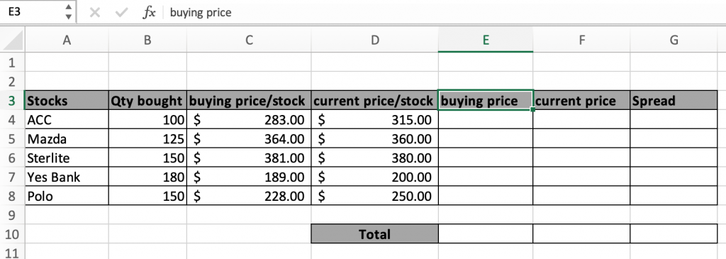
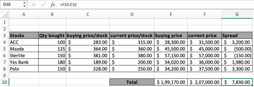
All of these might be confusing to understand. Let's understand how to use the function using an example. Here we have 5 stocks with their quantity, bought price/stock, current price/stock.
First we calculate ACC stocks bought for the data in the E4 cell.
Use the formula:
| =PRODUCT(B4,C4) |
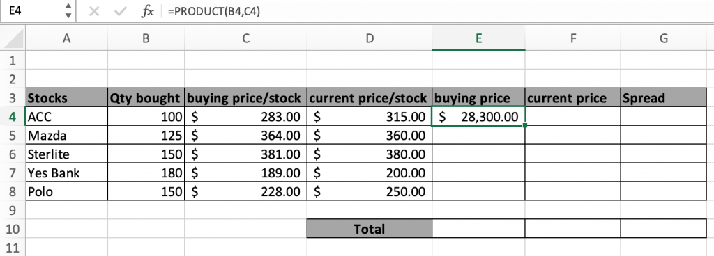
As you can see the total stock price spent on ACC. Now you can copy and paste this formula in E4 to further cells just by using Ctrl + C (copy) and Ctrl + V (Paste) or just by drag and drop the formula picking the box on the bottom right corner of the E4 cell.
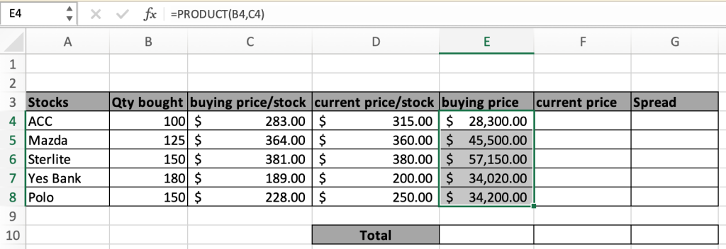
Now you can clearly see the amount spent on all stocks. Just get the Sum of all these values to get the total buying stocks.
Secondly we calculate the current price of the bought stocks. It means if we decide to sell at these prices.
Now we will use the same PRODUCT formula for the current price of ACC stocks in the F4 cell.
Use the formula:
| =PRODUCT(B4,D4) |
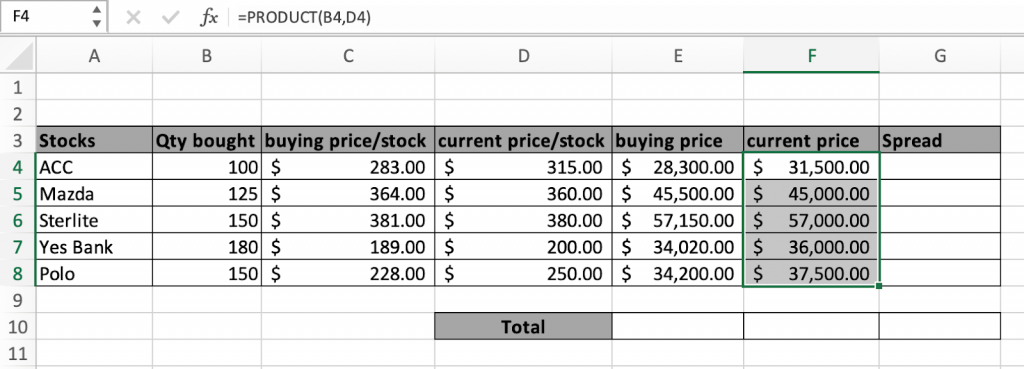
In the above snapshot it is clearly visible the current price of stocks.
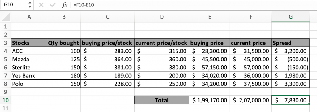
Now get the difference for all stocks in the Spread column
Use the formula:
| =PRODUCT(B4,D4) |
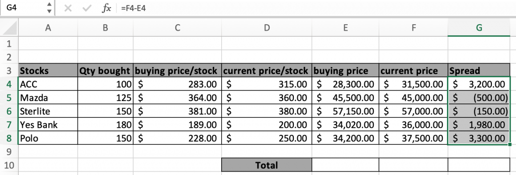
The amount in ( ) denotes the value is negative, it's just a currency format. Don't get confused. Now just get the sum to get the
Alternative Solution
The above process is used when you need to know the statistics for all different stocks. But you need to know the Statistics of the whole data, Use the SUMPRODUCT formula.
Use the formula:
| =SUMPRODUCT(B4:B8,C4:C8) |
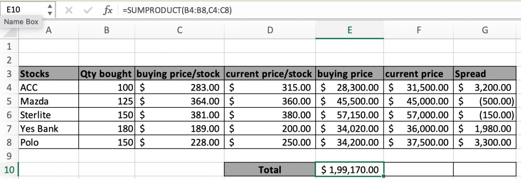
Now you can see in the above snapshot the total stock bought price.
Similarly we can calculate the total current price for the same stocks.
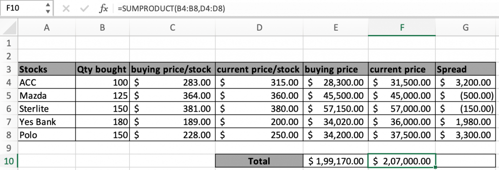
It's clearly visible if stocks are sold there is clearly some profit.
Get the difference of the two get the total profit
Here are all the observational notes using the SUM formulas in Excel
Notes :
Hope this article about How to Sum Stock Lists in Excel is explanatory. Find more articles on summing stocks and related Excel formulas here. If you liked our blogs, share it with your friends on Facebook. And also you can follow us on Twitter and Facebook. We would love to hear from you, do let us know how we can improve, complement or innovate our work and make it better for you. Write to us at info@exceltip.com.
Related Articles :
How to use the SUMPRODUCT function in Excel: Returns the SUM after multiplication of values in multiple arrays in excel.
SUM if date is between : Returns the SUM of values between given dates or period in excel.
Sum if date is greater than given date: Returns the SUM of values after the given date or period in excel.
2 Ways to Sum by Month in Excel: Returns the SUM of values within a given specific month in excel.
How to Sum Multiple Columns with Condition: Returns the SUM of values across multiple columns having condition in excel
How to use wildcards in excel : Count cells matching phrases using the wildcards in excel.
Popular Articles :
50 Excel Shortcuts to Increase Your Productivity : Get faster at your tasks in Excel. These shortcuts will help you increase your work efficiency in Excel.
How to use the IF Function in Excel : The IF statement in Excel checks the condition and returns a specific value if the condition is TRUE or returns another specific value if FALSE.
How to use the VLOOKUP Function in Excel : This is one of the most used and popular functions of excel that is used to lookup value from different ranges and sheets.
How to use the SUMIF Function in Excel : This is another dashboard essential function. This helps you sum up values on specific conditions.
How to use the COUNTIF Function in Excel : Count values with conditions using this amazing function. You don't need to filter your data to count specific values. Countif function is essential to prepare your dashboard.
The applications/code on this site are distributed as is and without warranties or liability. In no event shall the owner of the copyrights, or the authors of the applications/code be liable for any loss of profit, any problems or any damage resulting from the use or evaluation of the applications/code.


"Are you using the data in the example above?
If so, please can you post back with EXACTLY what you see in the formula bar in Excel (should start with an open curly bracket { as above), and what result you are getting. "
You can autosum with shorcut key alt+= in M.S. Excel
"I totally follow the instructions above but my results are
not as same as showed. The Part do not sum for all item, but sum only for the certain row.
What shold I do, I am assigned to prepare a worksheet which have the result of sum of each product like this.
Your advices would be so much meaning..."
A superb little trick that I had forgotten how to do - one of those useful tips that saves loads of file space and makes it easier to understand the calculation.