
In this article we will learn how we can make waterfall chart in Microsoft Excel 2010.
This chart is also known as the flying bricks chart or as the bridge chart. It’s used for understanding how an initial value is affected by a series of intermediate positive or negative values.
You can use this chart to show the revenue and expenditure of a business or even personal accounts.
Let’s take an example and understand how and where we can use this chart and how it will perform if we present the information in Water Fall Chart.
We have a data set where we have the revenue, cost of sales, etc. Now let’s insert another column before column B and enter “Remaining Profit” as the title.

This is calculated as follows
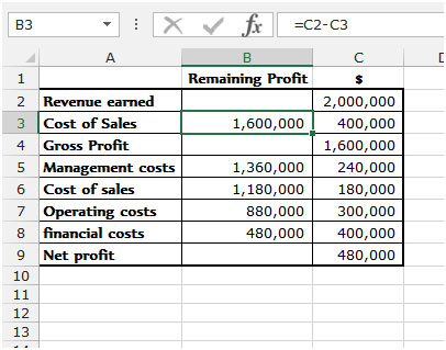
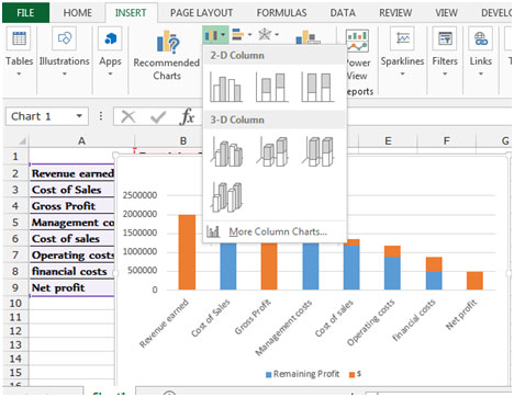
Now we just need to plot this and we will come up with an interesting looking waterfall chart.
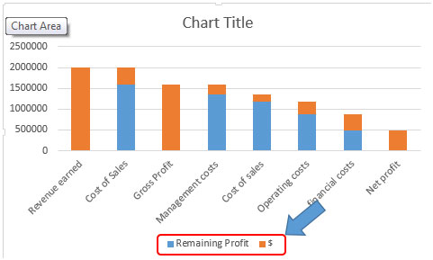
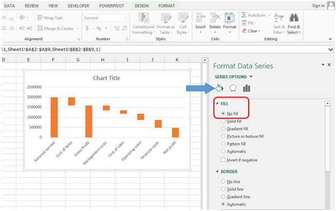
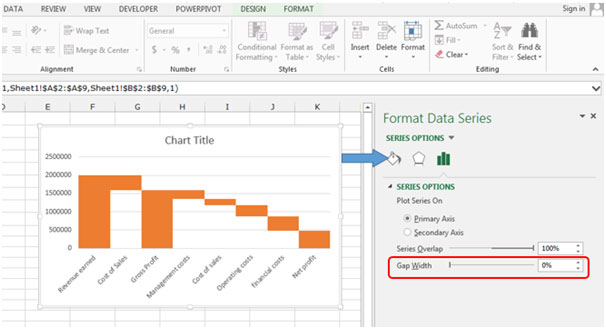
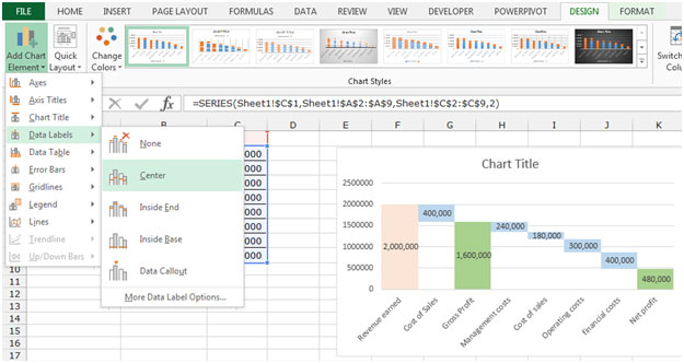
It’s almost done. Just a few things are left. Change the fill color of revenue earned, gross profit and net profit to a green. Now you can change the scale, add data labels, etc and format it further.
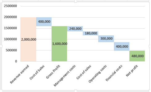
That’s it, a simple waterfall chart. This can be really useful when you want to include it in your reports and show data from a different angle.
Popular Articles:
50 Excel Shortcuts to Increase Your Productivity
How to use the VLOOKUP Function in Excel
The applications/code on this site are distributed as is and without warranties or liability. In no event shall the owner of the copyrights, or the authors of the applications/code be liable for any loss of profit, any problems or any damage resulting from the use or evaluation of the applications/code.


Great guide! But this way good for rare using of waterfall charts. If you create waterfall charts often and in large quantities, you should automate the creation process. You can do it easy if you install Waterfall Chart Studio Excel add-in.
By the way, waterfall charts become the standard type in Excel 2016. But if you use older version of Excel, Waterfall Chart Studio will be useful for you.
Wooooooooooow n Awesome guys
This is really interesting & step by step tutorial.
William