
In this article, we will learn how and where we can use Excel formula IFERROR.
IFERROR- This function is used when we get any error by using another formula or by doing the any calculation
The Syntax of IFERROR function: =IFERROR(Value,value_if_error)
Let’s take an example and understand how we can use Excel IFERROR formula.
We have fruits data in range A1:D6. Column A contains Fruits Name, Column B contains Kilograms, Column C contains Rate and in column D, we have returned the amount per kilogram.
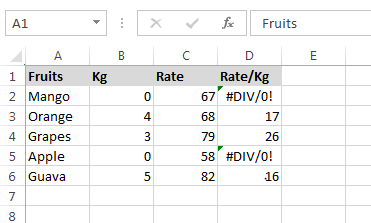
Where kilogram is zero the formula is giving #DIV/0! Error. We need a formula that can produce the result as 0 if the kilogram is zero, else show the rate per kilogram.
Follow below given steps:-
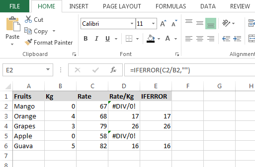
By Using IFERROR formula, we can ignore error while calculation in Microsoft Excel.
The applications/code on this site are distributed as is and without warranties or liability. In no event shall the owner of the copyrights, or the authors of the applications/code be liable for any loss of profit, any problems or any damage resulting from the use or evaluation of the applications/code.


