

In this article, we will learn How to Rank Salespeople According to Sales Figure in Excel.
Scenario :
In excel, ranking is used as statistics to show a relation. Ranking numbers is a very common and useful appendage when worming sales data. For example finding the top salesperson and lowest salesperson in the department. For problems like these we use the RANK formula in excel explained below with an example.
Rank formula in Excel
Rank function in excel takes two arguments first is the value itself and second is the array within ranking required. Learn how to use the RANK function in excel below.
Excel Rank formula
| =RANK(value, array, 0) |
value : value to rank
array : array in which to rank
Example :
All of these might be confusing to understand. Let's understand how to use the function using an example. Here we have some sales data to handle. First we rank all the values using the rank formula in excel.
Use the formula:
| =RANK(B2,sales,0) |
Here sales is fixed array B2:B6
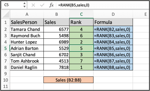
Copy and paste the formula to other cells using Ctrl + D. As you can see in the above image all the ranks with respective formulas. Now we can also sort the salesperson based on their respective rank or sales figure in excel.
Sort sales person using the sales figure
Sorting in excel can be done by Sort and filter option and can also be done using excel functions. Use the below formula to understand the new sorted sales person column.
Use the formula:
| =INDEX(person,MATCH(LARGE(sales,ROW(A1)),sales,0)) |
Here sales is fixed array B2:B6 and person is fixed array A2:A6
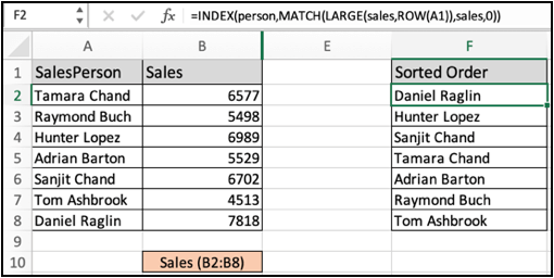
As you can see now you have another sorted column using excel functions. Now You have learnt how to sort columns based on the other columns.
Here are all the observational notes using the formula in Excel
Notes :
Hope this article about How to Rank Salespeople According to Sales Figure in Excel is explanatory. Find more articles on calculating values and related Excel formulas here. If you liked our blogs, share it with your friends on Facebook. And also you can follow us on Twitter and Facebook. We would love to hear from you, do let us know how we can improve, complement or innovate our work and make it better for you. Write to us at info@exceltip.com.
Related Articles :
How to use Shortcut Keys for Sort & filter in Excel : Use Ctrl + Shift + L from keyboard to apply sort and filter on table in Excel.
The SORT Function in Excel 365 (new version) : The SORT function returns the sorted array by the given column number in the array. It also works on horizontal data.
Sort numbers using Excel SMALL Function : To sort numbers using formula in Excel 2016 and older, you can use the SMALL function with other helping functions.
Sort Numeric Values with Excel RANK Function : To sort the numeric values we can use the Rank function. The formula is
Excel Formula to Sort Text : To sort text values using formula in excel we simply use the COUNTIF function. Here is the formula
Excel Formula to Extract Unique Values From a List : To find all unique values from a list in Excel 2016 and older versions, we use this simple formula.
UNIQUE Function for Excel 2016 : The Excel 2016 does not provide the UNIQUE function but we can create one. This UDF UNIQUE function returns all unique values from the list.
How To Count Unique Values in Excel With Criteria : To count unique values in excel with criteria we use a combination of functions. The FREQUENCY function is core of this formula
Popular Articles :
50 Excel Shortcuts to Increase Your Productivity : Get faster at your tasks in Excel. These shortcuts will help you increase your work efficiency in Excel.
How to use the VLOOKUP Function in Excel : This is one of the most used and popular functions of excel that is used to lookup value from different ranges and sheets.
How to use the IF Function in Excel : The IF statement in Excel checks the condition and returns a specific value if the condition is TRUE or returns another specific value if FALSE.
How to use the SUMIF Function in Excel : This is another dashboard essential function. This helps you sum up values on specific conditions.
How to use the COUNTIF Function in Excel : Count values with conditions using this amazing function. You don't need to filter your data to count specific values. Countif function is essential to prepare your dashboard.
The applications/code on this site are distributed as is and without warranties or liability. In no event shall the owner of the copyrights, or the authors of the applications/code be liable for any loss of profit, any problems or any damage resulting from the use or evaluation of the applications/code.


