

So before we learn how to do custom sort a Pivot table in Excel. Let's establish the basic meaning of custom sorting in Excel.
In Excel by default, the sorting is done numerically/alphabetically. For example, if you have a column with the name of months and you sort it, by default it will be sorted alphabetically (Apr,Feb,Jan…) instead of the order of the months. Same goes for pivot tables.
If you want to manual sort pivot tables with your own custom order, you need to tell that order to Excel. We had enough of the theory. Let's roll with an example.
Most of the businesses start their financial year from April and end in March. What we need to do is to custom sort our pivot table so that the report shows March as the first month, April as Second and so on.
So first create a pivot table by month. Here I have one pivot table that shows the sales done in different months.

Currently the pivot table is sorted in ascending order of months (because I have stored a list of months).
To custom sort my pivot table, I need to define the list. So in a range I write the order of the months I need.

Now, to add this list to excel, follow these steps.
Click on File. Go to option. Click on Advanced Option. Find the General category. Click on Edit Custom List.

The custom list dialog will open. You will see some predefined lists here. You can see we already have Jan, Feb, Mar… listed as a custom list. This is why my report is sorted by month.
Now to add our own custom list here, click in the input box below and select the range that contains your list. And click on import.

Note that we have an import button not added. It means the list will be static in the system. Making changes later in the range won't affect the list.

Click ok and get out of the settings.
Now try to sort the list by month.

You can see that the report is now sorted according to our given list instead of the default sorting method.
If it doesn't work, make sure that you have enabled sorting by custom list for Pivot table. To confirm this, do this:
Right click on the pivot table and click on the Pivot Table Options. Click on the total and filters tab on the open dialog box. Find Totals and Filters tab. Check the Use Custom List when sorting option.

And it is done.
Now you are ready to roll out your pivot report with custom sorted data.
Let’s take an example how we can create a pivot table report.
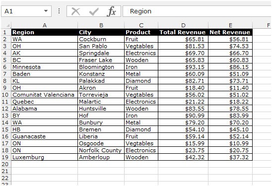
We have data in range A1:E19. Column A contains Region, column B contains City, column c contains product, column D contains total revenue and column E contains Net revenue.
Follow below given steps:-


This is the way to create pivot table report in Microsoft Excel.
Hope this article about How to use Pivot Table Report in Microsoft Excel is explanatory. Find more articles on pivot table formulas and related Excel formulas here. If you liked our blogs, share it with your friends on Facebook. And also you can follow us on Twitter and Facebook. We would love to hear from you, do let us know how we can improve, complement or innovate our work and make it better for you. Write to us at info@exceltip.com.
Related Articles:
subtotal grouped by dates in pivot table in Excel : find the subtotal of any field grouped by date values in pivot table using the GETPIVOTDATA function in Excel.
Pivot Table : Crunch your data numbers in a go using the PIVOT table tool in Excel.
Dynamic Pivot Table : Crunch your newly added data with old data numbers using the dynamic PIVOT table tool in Excel.
Show hide field header in the pivot table : Edit ( show / hide ) field header of the PIVOT table tool in Excel.
How to Refresh Pivot Charts : Refresh your PIVOT charts in Excel to get the updated result without any problem.
Popular Articles :
How to use the IF Function in Excel : The IF statement in Excel checks the condition and returns a specific value if the condition is TRUE or returns another specific value if FALSE.
How to use the VLOOKUP Function in Excel : This is one of the most used and popular functions of excel that is used to lookup value from different ranges and sheets.
How to Use SUMIF Function in Excel : This is another dashboard essential function. This helps you sum up values on specific conditions.
How to use the COUNTIF Function in Excel : Count values with conditions using this amazing function. You don't need to filter your data to count specific values. Countif function is essential to prepare your dashboard.
The applications/code on this site are distributed as is and without warranties or liability. In no event shall the owner of the copyrights, or the authors of the applications/code be liable for any loss of profit, any problems or any damage resulting from the use or evaluation of the applications/code.


Hello, I enjoy reading all of your post. I wanted to write a little comment to support you.
http://www.jarrowpomhealth.com
Fantastic post however I was wanting to know if you could write a litte more on this subject? I'd be very thankful if you could elaborate a little bit more. Cheers!
anglo-auto-leasing.org |